Use RoadRunner Scenario Object as Reference Oval Path

R2026b

This example shows how to import a RoadRunner Route (RoadRunner Scenario) object directly into the Reference Path Generator block and simulate a vehicle following that route. The block handles coordinate conversion and path resolution internally, generating the same oval path used in the Follow Waypoints Around Oval Track example.

This example requires RoadRunner and RoadRunner Scenario. For more information, see Install and Activate RoadRunner (RoadRunner).

The model includes a Simulation 3D Scene Configuration block for 3D visualization during simulation.

Open RoadRunner Project

In MATLAB®, start RoadRunner using the roadrunnerSetup (Automated Driving Toolbox) function. When the function opens a dialog box, specify the location of the RoadRunner installation folder and project folder. Update the installation and project paths to match your environment.

projectFolder = "C:\Projects\RoadRunner Project";
installFolder = "C:\Program Files\RoadRunner R2026a";

rrExe = fullfile(installFolder, "bin", "win64", "AppRoadRunner.exe");
system('"' + string(rrExe) + '" --project "' + string(projectFolder) + '" &');
pause(45);

Connect to RoadRunner and Create Oval Track Scenario Route

Establish a connection to the running RoadRunner instance and access the Scenario workspace.

rrApp = roadrunner.connect();

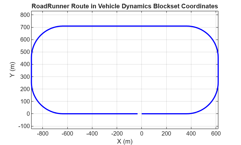
Define an oval track (stadium shape) matching the vdynblksOvalTrack model geometry: 1000 m top/bottom straights, 200 m side straights, 254.65 m corner radius, proceeding clockwise from the origin.

% Track parameters
straightLong = 1000;    % Top and bottom straight length (m)
straightShort = 200;    % Left and right straight length (m)
cornerRadius = 254.65;  % Quarter-circle corner radius (m)
numPtsPerCurve = 20;    % Waypoints per quarter-circle

% Curve centers (clockwise from top-right)
trCenter = [363.36, -254.65];
brCenter = [363.36, -454.65];
blCenter = [-636.64, -454.65];
tlCenter = [-636.64, -254.65];

Generate waypoints for each segment of the oval track. The track consists of 8 segments traversed clockwise: 4 straights connected by 4 quarter-circle arcs. Each straight is defined using linspace to distribute points evenly along the segment. Each curve is parameterized using the arc center and radius with angular samples from the entry angle to the exit angle (decreasing by 90° for clockwise traversal). The final waypoint array removes duplicate junction points where segments meet, then appends a zero Z-column for the 3-D coordinate required by drivingScenario.

n = numPtsPerCurve;

% Top straight (East): origin to top-right curve entry
seg1 = [linspace(0, trCenter(1), 11)', zeros(11,1)];

% Top-right curve: 90 deg CW
th = linspace(pi/2, 0, n)';
seg2 = [trCenter(1) + cornerRadius*cos(th), trCenter(2) + cornerRadius*sin(th)];

% Right straight (South)
seg3 = [repmat(trCenter(1)+cornerRadius, 11, 1), linspace(trCenter(2), brCenter(2), 11)'];

% Bottom-right curve: 90 deg CW
th = linspace(0, -pi/2, n)';
seg4 = [brCenter(1) + cornerRadius*cos(th), brCenter(2) + cornerRadius*sin(th)];

% Bottom straight (West)
seg5 = [linspace(brCenter(1), blCenter(1), 31)', repmat(brCenter(2)-cornerRadius, 31, 1)];

% Bottom-left curve: 90 deg CW
th = linspace(-pi/2, -pi, n)';
seg6 = [blCenter(1) + cornerRadius*cos(th), blCenter(2) + cornerRadius*sin(th)];

% Left straight (North)
seg7 = [repmat(blCenter(1)-cornerRadius, 11, 1), linspace(blCenter(2), tlCenter(2), 11)'];

% Top-left curve: 90 deg CW
th = linspace(pi, pi/2, n)';
seg8 = [tlCenter(1) + cornerRadius*cos(th), tlCenter(2) + cornerRadius*sin(th)];

% Return top straight (East): back toward origin
seg9 = [linspace(tlCenter(1), 0, 20)', zeros(20,1)];

% Combine segments (remove duplicate junction points)
ovalWaypoints = [seg1(1:end-1,:); seg2(1:end-1,:); seg3(1:end-1,:); ...
    seg4(1:end-1,:); seg5(1:end-1,:); seg6(1:end-1,:); ...
    seg7(1:end-1,:); seg8(1:end-1,:); seg9(1:end-1,:)];
ovalWaypoints3D = [ovalWaypoints, zeros(size(ovalWaypoints,1),1)];

Create a driving scenario, add the oval track road and an ego vehicle trajectory, and export to OpenSCENARIO format.

ds = drivingScenario;
road(ds, ovalWaypoints3D, 'Lanes', lanespec(1));
ego = vehicle(ds, 'ClassID', 1, 'Name', 'OvalVehicle');
trajectory(ego, ovalWaypoints3D, 30);

xoscFile = fullfile(tempdir, 'OvalTrack.xosc');
export(ds, "OpenSCENARIO XML", xoscFile);

Import the scenario into RoadRunner and save the scene.

newScenario(rrApp);
importScenario(rrApp, xoscFile, "OpenSCENARIO XML");
saveScene(rrApp, "OvalTrack.rrscene");
saveScenario(rrApp, "OvalTrack.rrscenario");

Access RoadRunner API and Extract Route

Access the Scenario workspace to retrieve the ego vehicle route object. The route contains position samples defining the oval track path. The Reference Path Generator block accepts Route (RoadRunner Scenario), Scenario (RoadRunner Scenario), or roadrunnerAPI (RoadRunner) objects directly in its refPathXY parameter.

rrApi = roadrunnerAPI(rrApp);
scenario = rrApi.Scenario;
egoRoute = scenario.Actors(1).InitialPoint.Route;

Visualize RoadRunner Path

Plot the route position samples to verify the oval track shape. RoadRunner uses a Y-left coordinate system while Vehicle Dynamics Blockset uses Y-right, so you must negate the Y coordinate for visualization in Vehicle Dynamics Blockset coordinates. This is the same oval path used in the Follow Waypoints Around Oval Track example.

posRR = egoRoute.PositionSamples;
xPath = posRR(:,1);
yPath = -posRR(:,2);

figure
plot(xPath, yPath, "b-", LineWidth=2)
xlabel("X (m)")
ylabel("Y (m)")
title("RoadRunner Route in Vehicle Dynamics Blockset Coordinates")
axis equal
grid on

Compute Initial Conditions and Configure Model

Extract the initial vehicle pose from the first route samples. Compute the heading angle from the tangent between the first two position samples, with Y negated for the Vehicle Dynamics Blockset coordinate frame.

x0 = posRR(1,1);
y0 = -posRR(1,2);
psi0 = atan2(-(posRR(2,2)-posRR(1,2)), posRR(2,1)-posRR(1,1));

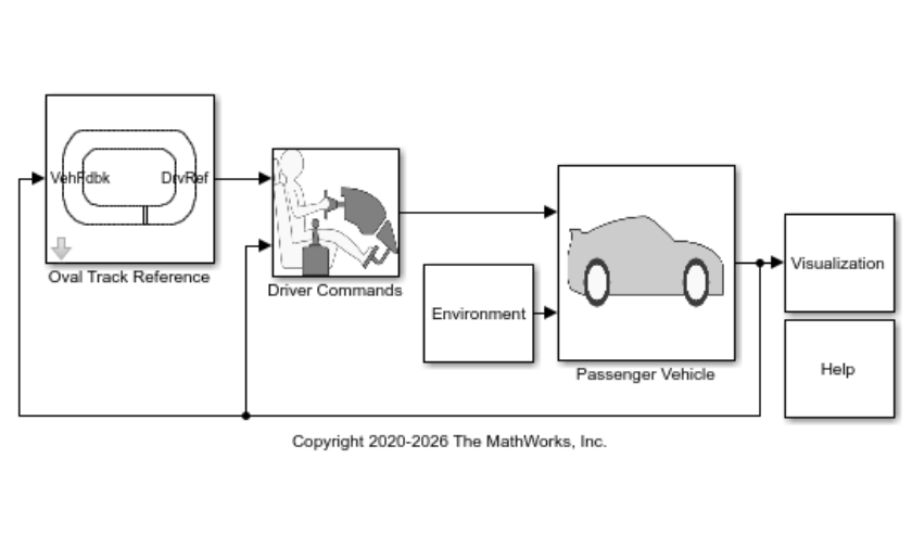
Open the vdynblksOvalTrack model. This model simulates a 3 degree-of-freedom (DOF) vehicle driving around a track. The Oval Track Reference subsystem contains a Reference Path Generator block that reads waypoints and outputs reference pose, curvature, and velocity signals. A Linear Predictive Driver steers the vehicle along the path, while a Powertrain and Driveline subsystem tracks the velocity command. The vehicle is modeled with a Vehicle Body 3DOF block.

Open the model and enable 3D visualization.

mdl = "vdynblksOvalTrack";
open_system(mdl)
set_param(mdl, "ReturnWorkspaceOutputs", "on");
set_param(mdl, "StopTime", "100");
set_param(mdl + "/Visualization/3D Visualization", "engine3D", "Enabled - Ground Following");
set_param(mdl + "/Passenger Vehicle/Vehicle Body 3DOF Dual Track/Light Logic/Lowbeam", "Value", "false");
simulinkScreenshot(mdl);

Configure the Reference Path Generator block. Set the refPathXY parameter to the workspace variable containing the RoadRunner route object. The block resolves the route to [X, Y, Yaw] waypoints at initialization, applying coordinate conversion automatically.

blk = mdl + "/Oval Track Reference/Reference Path Generator";
set_param(blk, "refPathXY", "egoRoute");
set_param(blk, "pathClosed", "on");
set_param(blk, "velRefMode", "Constant");
set_param(blk, "velRef", "100");
set_param(blk, "velRefUnit", "mph");
set_param(blk, "velLim", "off");

Set the vehicle initial conditions to match the starting pose of the route.

vehBlk = mdl + "/Passenger Vehicle/Vehicle Body 3DOF Dual Track/Vehicle Body 3DOF Dual Track";
set_param(vehBlk, "x_o", "x0");
set_param(vehBlk, "y_o", "y0");
set_param(vehBlk, "psi_o", "psi0");
set_param(vehBlk, "xdot_o", "44.704");

Simulate

Run the simulation. The Reference Path Generator resolves the RoadRunner route object into waypoints at model initialization and generates reference pose and velocity signals for the vehicle to follow at 100 mph around the oval track.

simOut = sim(mdl);

3D Visualization

The Simulation 3D Viewer shows the vehicle following the oval track at a constant 100 mph.

..\..\..\..\..\Desktop\image.mp4

Results

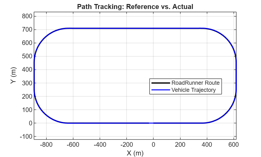
Extract the logged vehicle state signals and plot the actual vehicle trajectory against the reference path from RoadRunner.

logsout = simOut.logsout;
X1 = logsout.getElement("<X>");
Y1 = logsout.getElement("<Y>");

figure
plot(xPath, yPath, "k-", LineWidth=2)
hold on
plot(X1.Values.Data, Y1.Values.Data, "b-", LineWidth=1.5)
xlabel("X (m)")
ylabel("Y (m)")
title("Path Tracking: Reference vs. Actual")
legend("RoadRunner Route", "Vehicle Trajectory", Location="best")
axis equal
grid on

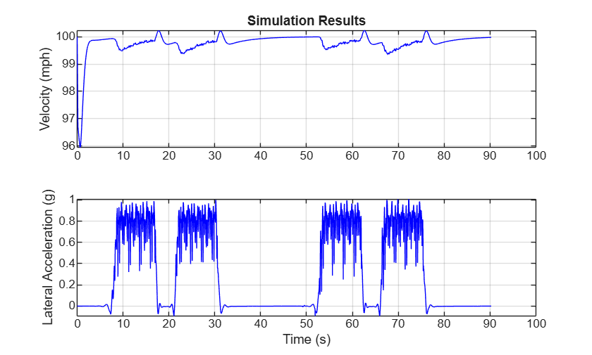
Plot longitudinal velocity in mph and lateral acceleration in g over time.

vel = logsout.getElement("xdot_mph");
ay = logsout.getElement("<ay>");

figure
subplot(2,1,1)
plot(vel.Values.Time, vel.Values.Data, "b-")
ylabel("Velocity (mph)")
title("Simulation Results")
grid on
subplot(2,1,2)
plot(ay.Values.Time, ay.Values.Data, "b-")
xlabel("Time (s)")
ylabel("Lateral Acceleration (g)")
grid on

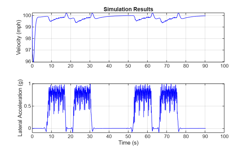
The velocity plot shows the vehicle reaching and maintaining approximately 100 mph on the straights. In the corners, the lateral acceleration spikes as the vehicle attempts to maintain the target speed through the 254.65 m radius curves. At 100 mph (44.7 m/s), the theoretical lateral acceleration on the curves is:

$$a_y=v^2/R=44.7^2/254.65\approx 0.8,\text{g}$$

The high lateral acceleration in the corners indicates that the vehicle is near the limits of tire grip, which can lead to path tracking degradation and potential loss of control.

Next Steps

To improve cornering behavior, enable curvature-based handling limits on the Reference Path Generator block. Handling limits automatically reduce the reference velocity before curves based on the path curvature and a specified maximum lateral acceleration so that the vehicle stays within tire grip limits. For an example, see Create and Use an Oval Track.