Overview of Traffic Models

In wireless network simulations, traffic models define how data flows between nodes, providing a framework to simulate different types of network usage and application behaviors. Among the various traffic models, four of most frequently used are On-Off, voice over internet protocol (VoIP), video conference and file transfer protocol (FTP).

• On-Off — Simulates both bursty and periodic transmissions depending on its configuration

• VoIP — Represents voice communication.

• Video Conference — Captures interactive audio and video traffic.

• FTP — Emulates bulk data transfers

With Wireless Network Toolbox™, you can implement these traffic models using the networkTrafficOnOff, networkTrafficVoIP, networkTrafficVideoConference, and networkTrafficFTP objects, respectively. The toolbox also supports custom traffic models through the wnet.Traffic base class for advanced or application-specific behaviors. This topic presents an overview of these traffic models.

On-Off Traffic Model

The On-Off traffic model represents network activity by switching between two distinct states: On and Off. In the On state, the system transmits data at a specified rate, while in the Off state, it sends no data. You can set the durations of each state using either fixed values or probabilistic distributions. By adjusting the On and Off durations and the data rate during the On state, you can simulate various real-world traffic patterns, such as periodic, bursty, or random traffic.

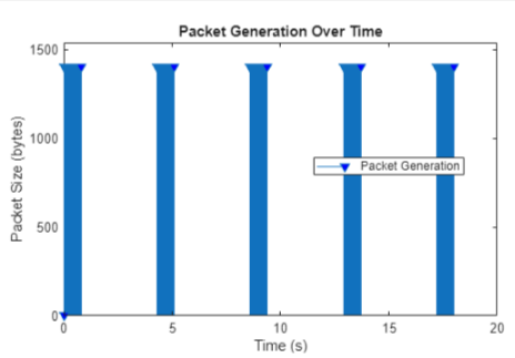
The figure shows how the On-Off model operates. During the On state, the model generates packets at fixed intervals. Typically, the On and Off state durations follow exponential distributions with mean values of OnExponentialMean and OffExponentialMean, respectively.

Periodic Traffic

Periodic traffic refers to the transmission of data packets at consistent, predetermined time intervals. Typical examples include sensors that send readings at regular intervals, heartbeat signals exchanged in a distributed system, and scheduled updates in automated control systems.

For an example of how to generate periodic traffic, see Periodic Traffic.

Bursty Traffic

Bursty traffic involves short periods of intense activity followed by longer gaps of silence. You can model this by choosing a short On duration with a high data rate, followed by a longer Off duration. This reflects traffic patterns typical in video streaming or large file downloads.

For an example of how to generate bursty traffic, see Bursty Traffic.

Random Traffic

Random traffic refers to data transmissions that occur at irregular and unpredictable intervals. The timing of active and idle periods varies, often based on statistical distributions like the exponential distribution.

For an example of how to generate random traffic, see Random Traffic.

VoIP Traffic in IEEE 802.11ax

VoIP enables you to carry real-time voice conversations over data networks such as Wi-Fi. Unlike data downloads, VoIP traffic flows in both directions between the user device (STA) and the access point (AP), since both parties speak and listen during a call. This creates bi-directional and symmetric traffic.

The nature of human conversation means that people do not talk continuously. Instead, speech consists of alternating periods of talking and silence. IEEE^® 802.11ax™ models this behavior using a two-state Markov model: one state represents active talking, the other represents silence. At any given time, the VoIP user is in either the talking state (State 1) or the silence state (State 0), as shown in these figures.

These probabilities govern the transition between states:

• A person in the talking state goes silent with probability a.

• A person in the silence state starts talking with probability b.

• The probability of staying in the same state is $$1-a$$ for talking and $$1-b$$ for silence.

This state update happens at a regular rate determined by the speech encoder. The encoder processes speech in frames, and each frame corresponds to a small time interval. For talking, the frame duration is typically 20 milliseconds. For silence, the frame duration is longer (160 milliseconds) since less information is sent.

The durations of talking and silence periods are modeled using exponential distributions. That means most periods are short, but occasionally longer bursts occur. The exponential distribution is mathematically defined as

$$\text{f}\left(t\right)＝\lambda e^{\left(-\lambda t\right)}$$, $$t\ge 0$$.

Here, λ is the rate parameter. For talk spurts, this rate might be higher (shorter durations), while for silence, it is lower (longer durations). The exponential distribution is memoryless, meaning the chance of continuing or ending a state does not depend on how long you have already been in that state. This matches natural speech patterns well.

The system generates VoIP packets at the end of each frame, but with a small random delay called jitter, τ. As a result, the actual packet generation time is $$iT+\tau$$, where i is the frame index and T is the frame duration. During the talking state, the system generates packets at short, regular intervals. During silence, packets are fewer and smaller.

This jitter arises due to network delays, and is modeled using a Laplace distribution, which accounts for both early and late arrivals. The Laplace distribution has two parameters:

• μ — the average delay (often set to 0)

• b — A scale that controls how widely delays vary

The equation for this distribution is: $$\begin{array}{l} \\ f_J\left(j\right)=\left(\frac{1}{2b}\right)e^{\left(-\frac{\left|j-\mu \right|}{b}\right)}\end{array}$$

Video Conference Traffic Model

Video conferencing traffic is different from simple downloads or web browsing. It is continuous, real-time, and involves high variability in data sizes and delay. IEEE 802.11ax [3] defines a traffic model to simulate this realistically using the Weibull and gamma distributions.

• Weibull distribution — Used to model the sizes of video frames

• Gamma distribution — Used to model the network latency experienced by packets

Generate Video Frames

A video encoder captures the speaker's face or shared screen and generates video frames (snapshots of the scene). These are generated periodically (for example, 30 frames per second means it generates one frame every 33.3 ms). However, the sizes of these frames are not constant. Frame sizes in a video conference vary because the amount of motion in the scene affects how much data is required to represent each frame. When there is low motion, such as a person sitting still and talking, the video encoder can compress the image more efficiently, resulting in smaller frame sizes. In contrast, high motion, like hand movements or screen sharing with frequent changes, requires more data to maintain quality, leading to larger frame sizes. You can model this natural variation using the Weibull distribution, which captures the tendency for most frames to be small with occasional large ones.

These equations represent the probability density function of the Weibull distribution.

$$\begin{array}{l}\text{}\\ f\left(x;k,\lambda \right)=\left(\frac{k}{\lambda }\right){\left(\frac{x}{\lambda }\right)}^{\left(k-\text{1}\right)}{e}^{-{\left(\frac{x}{\lambda }\right)}^k},x\ge 0\end{array}$$​

$$f\left(x;k,\lambda \right)=0$$,​ $$x<0$$.​

Here, x is the frame size in bytes, k is the shape parameter (which controls the skewness), and λ is the scale parameter (which controls average size).

This table provides the scale and shape parameters based on the video bit rate.

Video Bit Rate	λ	k
2 Mbps	6950	0.8099
4 Mbps	13900	0.8099
6 Mbps	20850	0.8099
8 Mbps	27800	0.8099

Network Latency

Packets experience delay as they travel through the network. This delay is not fixed, and varies due to queuing, congestion, and wireless contention. IEEE 802.11ax models this using the gamma distribution.

This represents the probability density function of the gamma distribution:

$$f\left(\text{x};\text{k},\theta \right)=\frac{\left(x^{k-1}{e}^{-\left(\frac{x}{\theta }\right)}\right)}{\Gamma (k){\theta }^k}$$​, ​$$x\ge 0$$.

$$f\left(\text{x};\text{k},\theta \right)=0$$,​ $$x<0$$.

Here, x is the delay (latency) in milliseconds, k is the shape parameter, and Γ(k) is the gamma function. With values of k＝0.2463 and θ＝60.227, the mean latency is 14.834 ms. To increase or decrease network latency, adjust θ linearly, since the mean of a gamma distribution equals kθ.

FTP Traffic Model:

FTP traffic refers to file transfer behavior over a network and is modeled as a sequence of file transmissions separated by periods of inactivity known as reading time. In this model, each file transfer corresponds to a packet call, where the packet call size is equal to the file size (S). The reading time (D) is defined as the time between the end of one file transmission and the start of the next, effectively serving as the inter-arrival time between successive packet calls.

Local FTP Traffic Model

The Local FTP Traffic Model represents typical file download behavior in indoor wireless networks, such as enterprise or home settings. This model is part of the 802.11ax Evaluation Methodology for assessing the performance of Wi-Fi 6 systems.

Traffic Parameters

• File size (S) — Size of the file to be downloaded. The file size follows a truncated log-normal distribution. The 802.11ax, standard uses parameters like μ＝14.45 and σ＝0.35, and truncates file sizes within a specific range to avoid extremely large values.

• Reading time (D) — Time between the end of one file transfer and the start of the next. The reading time follows an exponential distribution and captures the random think-time between downloads ($${\text{f}}_{\text{D}}\left(\text{d}\right)=\lambda {\text{e}}^{-\left(\lambda d\right)}$$, $$d\ge 0$$). For example, if λ＝0.006, then $$\text{E}\left[D\right]＝\frac{1}{\lambda }=166.7$$ seconds.

• Packet arrival — During file transfer, the network sends packets at regular intervals. In 802.11ax , the network sends packet inter arrival time and reading time are same.

FTP Traffic Model 2 (3GPP)

FTP traffic model 2, as specified by 3GPP, is a simplified file transfer model used for evaluating mobile network performance. In this model, each user transfers files of a fixed size of 0.5 MB. The reading time between the end of one file transfer and the start of the next is modeled as an exponential distribution with a rate parameter of 0.02, resulting in a mean reading time of 50 seconds. The packet call size is fixed at 0.5 MB, and the inter-arrival time between packet calls is equal to the reading time.

FTP Traffic Model 3 (3GPP)

FTP traffic model 3, as specified by 3GPP, simulates file transfers for mobile network performance evaluation. In this model, each user transfers 0.5 MB files. The inter-arrival time, defined as the sum of transmission and reading times, follows an exponential distribution based on a Poisson process.

Custom Traffic Model

A custom traffic model is a user-defined pattern for generating network traffic in simulations or tests, tailored to specific requirements rather than using standard, prebuilt models. For instance, if you want to study how wireless local area network (WLAN) sensing traffic affects overall network performance, you can develop a tailored traffic model that accurately represents the behavior of sensing applications. You can use the wnet.Traffic base class from the Wireless Network Toolbox to implement your custom sensing traffic model.