Beamscan Direction of Arrival Estimation Using FPGA

This example uses:

This example shows how to use beamscan technique to estimate direction of arrival (DOA) in Simulink®. This example is based on the Direction of Arrival with Beamscan and MVDR example.

This example simulates the reception of two narrowband incident signals on a 10-element uniformly linear antenna array (ULA). A DOA algorithm cannot uniquely determine azimuth and elevation for a linear array, so it returns a calculation of broadside angles to represent apparent direction. In this example, because the elevation of the sources is at 0 degrees and the scanning region is from -90 to 90 degrees, the broadside and azimuth angles are the same. The model simulates reception of the source signals with added noise, and calculates the beamscan spatial spectra.

Beamscan Algorithm

The algorithm used in the beamscan estimator examples in Phased Array System Toolbox™ has many other names and descriptions but is fundamentally a simple matrix multiplication followed by a scalar multiplication and summation.

The first step in the algorithm is computing the spatial covariance matrix, which you do by cross-multiplying each of the input antenna signals by the conjugate of every other antenna signal. Since there are 10 antenna elements, there are 55 total combinations. You then sum these cross products over some number of samples that you have to determine.

For a 10-element ULA and 181 azimuth directions (-90 degrees to +90 degrees, including 0 degrees), you must first pre-compute the 181-by-10 matrix of steering vectors. For this calculation, create a phase.SteeringVector object and pass it the vector of scanning angles [-90:90]. The object returns a 10-by-181 matrix.

You need the Hermitian transpose of that matrix formed by taking the conjugate and reshaping the matrix to be 181-by-10. Then, matrix-multiply the Hermitian transpose by the 10-by-10 spatial covariance matrix, which is a 181-by-10 result.

To get the real-only power estimate, you then point-multiply each result from the previous matrix multiplication by the elements of the steering vector. This calculation results in a new 181x10 matrix which you sum along the second dimension, resulting a 181-element vector. In theory, multiplying by both the Hermitian (conjugated) and normal versions of the steering vector should result in a real-only result, but small round-off errors can occur and dropping the imaginary part of the vector ensures a real-only final vector.

Exploring the Model

Open the model to start exploring.

modelName = 'DirectionOfArrivalHDLModel';
open_system(modelName);
set_param(modelName,'SampleTimeColors','on');
set_param(modelName,'SimulationCommand','Update');
set_param(modelName,'Open','on');
set(allchild(0),'Visible','off');

Test Bench Environment

The environment for the beamscan algorithm testing starts with two random sources that simulate the return signals from two targets of the RADAR. The position in azimuth and elevation of these two targets is set by the Position subsystem and the targets start at -20 degrees and 40 degrees azimuth. Every 1024 cycles, the start angles update such that the -20 degree bearing increases 3 degrees and the 40 degree bearing decreases 2 degrees. The elevation of both simulated targets remains at 0 degrees. In this example, the timing of the source movements is aligned with the hardware frame calculation, but in a more realistic simulation the spatial changes would not be aligned which would result in spreading of the estimated DOA.

open_system([modelName,'/Position']);

Receiver Array and Preamplifier

The sources and angles are passed to the Narrowband Rx Array block which, in addition to the operating frequency and the speed of light, takes the 10-element linear antenna array as a parameter. The resulting 10-element vector is sent to the Receiver Preamp block where a small amount of thermal noise for each antenna element is added.

The output from the Receiver Preamp then goes to an Unbuffer block to convert the frames of 1024-by-10 samples to a vector of 10 samples at a rate 1024 times faster. The final part of the environment models the ADC by converting the vector from double-precision to fixed-point values with a word-length of 12 bits and a fraction-length of 9-bits.

The resulting fixed-point vector is then sent to the HDLDOA subsystem, which is the part of the design that will go on the FPGA. A continuously high valid input is also provided to the HDLDOA subsystem.

Results from the HDLDOA subsystem are returned as a vector of 181 16-bit fixed-point real-only values that show the return amplitude for each of the 181 azimuth directions, from -90 to +90 degrees. This vector is then sent to an Array Plot scope to vizualize the spatial spectrum.

Choosing the Number of Parallel Calculations

The number of samples you choose to sum over for the covariance matrix is a critical parameter in running this algorithm in an FPGA. Consider the number of operations in the matrix multiply and point-multiply and the number of cycles needed to perform these operations. Assuming pipelined operation of one-clock-cycle multipliers, the 181-by-10 Hermitian-transposed steering vector multiplied by the 10-by-10 covariance matrix takes around 100 clock cycles plus some pipeline start-up latency.

Since the zero-degree steering vector is all-ones, you can replace the multipliers for this direction with a special case that adds all the entries in the covariance matrix. This simplification reduces the matrix size to 180-by-10.

You cannot fit the entire matrix multiplication in today's FPGAs in fully parallel form, so you must decide how to divide-and-conquer the computation. With 180 steering vectors, the factors of 180 such as 9, 10, 18, or 20 would be good choices for parallel calculations. Each parallel branch requires 11 complex multipliers, 10 for the matrix multiplication and one for the point-multiply that follows, and each complex multiplier requires either 3 or 4 real multipliers. Additionally, each multiplier can map to many DSP slices or blocks in an FPGA depending on word-length. Each parallel branch also requires an accumulator to create the final value for each matrix output.

It is useful to take a longer amount of time in the first step of creating the covariance matrix than the next matrix multiply stage, so that the next stage is always ready for data when results of the first step are ready, and no samples are dropped.

If you choose to do 9 steering vectors in parallel, then you would do twenty groups of 9 each, taking 2000 cycles plus some latency. You would then choose 2048 as the number of samples to sum over since that is slightly longer than the time required for the matrix multiplication.

If instead you choose to do 20 steering vectors in parallel, you would then need more multipliers but the 9 groups would only take 900 cycles plus latency so you could choose 1024 as the number of samples to sum over.

This example shows 18 steering vectors in parallel (10 groups of 18 vectors) which takes 1000 cycles plus latency and also leads to summing over 1024 samples.

FPGA Implementation

The first step of the algorithm is to compute the covariance matrix, which requires 55 complex multiplications and accumulators, and a counter to track the timing for each 1024 samples. Using a For-Each subsystem allows you to create one pipelined multiplier and accumulator and then repeat this operation 55 times.

open_system([modelName,'/HDLDOA/CovarianceCalc']);

Covariance Calculation

Calculating the indexes of which input is multiplied by which other inputs is best handled outside the For-Each subsystem. Selector blocks for each input to the multiplier create constant vectors as input to For-Each subsystem. These Selector blocks and constants are implemented as wiring connections in the final FPGA and do not consume FPGA fabric resources.

Once the 55 outputs are accumulated, a valid output signal indicates that the 1024 samples have been processed. The next step is to form the 10-by-10 covariance matrix from the 55 values using the conjugate operator. The conjugate operation creates a vector of 110 values that are the 55 original values and their conjugates. A Matrix Concatenation block and Selector blocks manages the indices needed to form this matrix and put each element in the vector into their proper location. Again, these connections are all wiring in the FPGA and use no FPGA fabric resources. The FIR filter that performs the inner-product calculation downstream requires the covariance matrix flipped up-down, so for convenience later, flip it here. There is no area cost for this flip, either. A covDone signal starts the next part of the algorithm and after that signal is asserted, the covariance matrix accumulation can restart with no loss of data.

Once the full covariance matrix is registered and the valid pulse is sent, the matrix multiplication phase can start. The startCtrl subsystem returns the runOut signal while this phase is running and clears this signal when this phase is complete. A second output signal controls the initial loading of the accumulators in the matrix multiply. The startCtrl subsystem also enforces an 8-cycle delay at start-up to avoid spuriously starting the matrix multiply phase, and does not allow a valid pulse from the covariance section if the matrix multiply is already running. This control protects the currently running calculation from a potential overflow.

The timing control of the matrix multiplication is divided into the input side of the FIR filter and the output side of the FIR filter. The input side handles the control for when to load the completed inner-product into a register and when to load the appropriate steering vector value for the point-multiply.

open_system([modelName,'/HDLDOA']);

Steering Vector ROMs

The steering vectors are stored in 18 ROMs in the ROMFIRMatMul subsystem. All of these ROMs have output registers with the ResetTypeHDL property set to none for better inference in synthesis. The ROM holds the quantized steering vectors in a 12-bit word-length data type to get good numeric performance. The ROM outputs are then sent to the FIR filter and point-multiply subsystems. Using the Discrete FIR Filter block to compute the inner-product provides high-performance complex multiplication and summation with little design effort.

open_system([modelName,'/HDLDOA/ROMFIRMatMul']);

Matrix Multiplication using FIR Filters

Each FIRMatMul subsystem registers some inputs to time-align signals from the ROM and includes a small FIFO that captures the steering vector value that is used for the point-multiply. This storage needs to be a FIFO and not a register for the case where the end of one round is followed by the beginning of the next round such that two values must be stored temporarily. The point-multiply is accomplished with a single external complex multiplier that then feeds into the accumulator. Since the final result is real-only, the imaginary part is dropped after the point-multiply.

The fixed-point settings of the FIR Filter can be left at the default values but the point-multiply prior to the accumulator is a good spot to control the bit-growth by quantizing to a 16-bit type. This quantization allows for a smaller accumulator. Depending on your application, if lower area in the FPGA is needed, you could quantize the results of the FIR Filter too.

open_system([modelName,'/HDLDOA/ROMFIRMatMul/FIRMatMul']);

Forming the Final Output

The output of the ROMFIRMatMul subsystem is a vector of 18 real-only results, but the model must store 10 groups of these to get the final result. This storage happens in the Output Reg Bank subsystem outside of the HDL part of the model. This subsystem tracks which group is being stored and produces a final valid output signal. The zero-degree steering vector result, which is calculated separately without multipliers, is also grouped here with the other results. A final output register stores the 180 results, one per degree of azimuth, as the final result. In your real system, this storage could be handled by software by sending the results to DRAM.

Simulating the Model

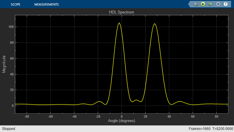
You can simulate the model by clicking the Run button or by using the command below. The simulation runs for a bit more than eight frames of 1024 samples, and so the results for six frames are shown on the HDL Spectrum block from -90 to +90 degrees azimuth. Since it takes approximately 2048 cycles to calculate the spectrum, only the results from six frames are shown. As you can see, the two targets are detected and their azimuth directions established.

sim(modelName);

Synthesizing the `HDLDOA` Subsystem

Running synthesis for the HDLDOA subsystem shows that the achievable clock rate in an AMD xc7vx485tffg1157-1 is around 100 MHz and the design consumes about 66,000 LUTs and 1408 DSP48 slices. The critical path goes through the point multiplier after the matrix multiply. The DSP48 slices can be broken down in to 55 subsystems each with 4 DSP48s, which is 220 for the complex multipliers in the CovarianceCalc subsystem. There are then 1188 DSP48 slices in the 18 subsystems that make up the ROMFIRMatMul subsystem. Each FIR and point-multiply uses 66 DSP48s for 10 complex filter taps and point-multiplier. The data types used here are large to help minimize errors but the accumulated result is quantized back to much smaller word-length. You can trade-off the quantization and number of multipliers used in the FIR-based matrix multiply to get the level of numerical accuracy you want to achieve.

Conclusion

You created a beamscan direction of arrival model for an FPGA that processes input from a 10-element uniform linear antenna array and produces the returned power for each of 181 compass directions, 18 at a time.

Going further, you could try reworking the model for a different number of parallel paths in the matrix multiplier section or you could change the number of antenna elements in the array. You could change the model to use a different number of steering vectors. You could experiment with fixed-point settings to get a lower area.