Accelerate Ray Tracing Analysis Using GPU

Since R2025a

This example shows how to accelerate the calculation of ray tracing propagation paths, signal strengths, and coverage maps by using a GPU. In general, to perform ray tracing analysis using a GPU, set the UseGPU property of a RayTracing propagation model object to "on". Then, use the RayTracing object as input to a ray tracing function such as raytrace, sigstrength, or coverage.

Using a GPU can accelerate ray tracing analysis when the GPU meets these conditions:

• The GPU includes dedicated ray tracing cores.

• The GPU outperforms the CPU on single-precision floating-point operations.

• The GPU has sufficient memory to accommodate the complexity of the scene and the requirements of the ray tracing model. You can change the requirements of the ray tracing model by setting properties of the RayTracing object.

Within the example:

• Verify that a GPU is available for computation.

• Create a scene by importing buildings into Site Viewer.

• Configure a ray tracing propagation model.

• Perform ray tracing analysis using the local CPU and then the GPU.

• Compare the results from the CPU and the GPU.

Ray tracing analysis with a GPU requires Parallel Computing Toolbox™ and a supported GPU device. For more information about supported devices, see GPU Computing Requirements (Parallel Computing Toolbox).

Check GPU Setup

Verify that a supported GPU is available for computation. Display the name of the GPU.

gpu = gpuDevice;
disp(gpu.Name + " GPU detected and available.")

NVIDIA RTX 4000 SFF Ada Generation GPU detected and available.

Note that the GPU used in this example has 48 ray tracing cores.

Create Scene

Specify the name of an OpenStreetMap file [1] that contains building data for Hong Kong. Create two scenes by importing the buildings into Site Viewer objects.

filename = "hongkong.osm";
viewerCPU = siteviewer(Buildings=filename,Name="Viewer for CPU Calculations");
viewerGPU = siteviewer(Buildings=filename,Name="Viewer for GPU Calculations");

Create a transmitter site and a receiver site.

tx = txsite(Name="Small cell transmitter", ...
    Latitude=22.2789, ...
    Longitude=114.1625, ...
    AntennaHeight=10, ...
    TransmitterFrequency=28e9);

rx = rxsite(Name="Small cell receiver", ...
    Latitude=22.2799, ...
    Longitude=114.1617, ...
    AntennaHeight=1);

Create Ray Tracing Models

Create two ray tracing propagation models, which MATLAB® represents using RayTracing objects.

• For both models, find propagation paths with up to 3 surface reflections and up to 1 edge diffraction.

• For both models, launch more rays than the default model by setting the AngularSeparation property to "low".

• For the first model, use the local CPU, which is the default option. For the second model, use the GPU by setting the UseGPU property to "on".

% CPU model
pmCPU = propagationModel("raytracing", ...
    MaxNumReflections=3, ...
    MaxNumDiffractions=1, ...
    AngularSeparation="low");

% GPU model
pmGPU = pmCPU;
pmGPU.UseGPU = "on";

Calculate Propagation Paths

Find propagation paths between the sites using the CPU and the GPU. Compare the results by viewing the propagation paths and the run times.

Use CPU

Calculate the propagation paths using the CPU and return the result as a cell array of comm.Ray objects. Measure the run time by using the tic and toc functions.

tStartCPU = tic;

% find paths using CPU
raysCPU = raytrace(tx,rx,pmCPU,Map=viewerCPU);

runTimeCPU = toc(tStartCPU);

Extract the propagation paths from the cell array.

raysCPU = raysCPU{1};

Use GPU

Calculate the propagation paths using the GPU and measure the run time.

tStartGPU = tic;

% find paths using GPU
raysGPU = raytrace(tx,rx,pmGPU,Map=viewerGPU);

runTimeGPU = toc(tStartGPU);

Extract the propagation paths from the cell array.

raysGPU = raysGPU{1};

Compare Results

Display the sites and the propagation paths in each Site Viewer by using the plotSitesAndRays helper function. The helper function is defined at the end of the example. Note that the propagation paths found by the GPU are practically indistinguishable from the propagation paths found by the CPU.

plotSitesAndRays(viewerCPU,raysCPU,tx,rx)
plotSitesAndRays(viewerGPU,raysGPU,tx,rx)

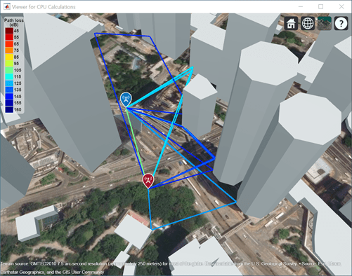
Compare the number of rays found by the CPU and the GPU.

numRaysCPU = numel(raysCPU);
numRaysGPU = numel(raysGPU);
fprintf("Number of CPU Rays: " + numRaysCPU + "\n" + ...
    "Number of GPU Rays: " + numRaysGPU + "\n")

Number of CPU Rays: 15
Number of GPU Rays: 15

Compare the run times for the CPU and the GPU.

speedUpFactor = runTimeCPU / runTimeGPU;
fprintf("CPU Time (s): " + runTimeCPU + "\n" + ...
    "GPU Time (s): " + runTimeGPU + "\n" + ...
    "Speed-up Factor: " + speedUpFactor)

CPU Time (s): 54.4435
GPU Time (s): 15.1039
Speed-up Factor: 3.6046

Calculate Signal Strength

Calculate the signal strength at the receiver site due to the transmitter site using the CPU and the GPU. Compare the results by viewing the signal strengths and the run times.

Use CPU

Calculate the signal strength using the CPU and measure the run time.

tStartCPU = tic;

% find signal strength using CPU
ssCPU = sigstrength(rx,tx,pmCPU,Map=viewerCPU);

runTimeCPU = toc(tStartCPU);

Use GPU

Calculate the signal strength using the GPU and measure the run time.

tStartGPU = tic;

% find signal strength using GPU
ssGPU = sigstrength(rx,tx,pmGPU,Map=viewerGPU);

runTimeGPU = toc(tStartGPU);

Compare Results

Compare the signal strengths calculated by the CPU and the GPU. Note that, due to small differences in algorithms and hardware implementations, the CPU and GPU models can return different results.

fprintf("CPU Signal Strength (dBm): " + ssCPU + "\n" + ...
    "GPU Signal Strength (dBm): " + ssGPU + "\n" + ...
    "Difference in Signal Strengths (dB): " + abs(ssCPU - ssGPU))

CPU Signal Strength (dBm): -65.0323
GPU Signal Strength (dBm): -65.0324
Difference in Signal Strengths (dB): 2.3394e-05

Compare the run time for the CPU and the GPU.

speedUpFactor = runTimeCPU / runTimeGPU;
fprintf("CPU Time (s): " + runTimeCPU + "\n" + ...
    "GPU Time (s): " + runTimeGPU + "\n" + ...
    "Speed-up Factor: " + speedUpFactor)

CPU Time (s): 54.6174
GPU Time (s): 15.151
Speed-up Factor: 3.6049

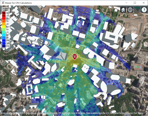
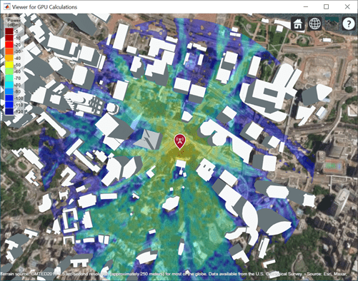
Calculate Coverage Map

Create a coverage map for the transmitter site using the CPU and the GPU. Compare the results by viewing the coverage maps and the run times.

Prepare to create the coverage maps by clearing the existing visualizations from each Site Viewer.

clearMap(viewerCPU)
clearMap(viewerGPU)

Use CPU

Create the coverage map using the CPU and measure the run time.

tStartCPU = tic;

% calculate coverage map using CPU
coverage(tx,pmCPU,SignalStrengths=-120:-5,Map=viewerCPU)

runTimeCPU = toc(tStartCPU);

Use GPU

Create the coverage map using the GPU and measure the run time.

tStartGPU = tic;

% calculate coverage map using GPU
coverage(tx,pmGPU,SignalStrengths=-120:-5,Map=viewerGPU)

runTimeGPU = toc(tStartGPU);

Compare Results

Compare the coverage maps created by the CPU and the GPU. Note that the coverage map created by the GPU is similar to the coverage map created by the CPU.

Compare the run time for the CPU and the GPU.

speedUpFactor = runTimeCPU / runTimeGPU;
fprintf("CPU Time (s): " + runTimeCPU + "\n" + ...
    "GPU Time (s): " + runTimeGPU + "\n" + ...
    "Speed-up Factor: " + speedUpFactor)

CPU Time (s): 5492.9788
GPU Time (s): 4321.6296
Speed-up Factor: 1.271

Note that the speed-up factor for point-to-point analysis functions such as raytrace and sigstrength can be larger than the speed-up factor for point-to-area analysis functions such as coverage.

Helper Functions

The plotSitesAndRays helper function displays the specified propagation paths and antenna sites in the specified Site Viewer.

function plotSitesAndRays(viewer,rays,tx,rx)
    show(tx,Map=viewer)
    show(rx,Map=viewer)
    plot(rays,Map=viewer)
end

References

[1] The OpenStreetMap file is downloaded from https://www.openstreetmap.org, which provides access to crowd-sourced map data all over the world. The data is licensed under the Open Data Commons Open Database License (ODbL), https://opendatacommons.org/licenses/odbl/.