Analyze Ambisonic Decoders
In this example, you derive objective metrics to analyze the performance of an ambisonic decoder.
You consider the following metrics:
Amplitude spread.
Energy spread.
Velocity vector magnitude and direction.
Energy vector magnitude and direction.
Apparent source width.
You use these metrics to understand the effect of loudspeaker placement on ambisonic decoding, and to compare different ambisonic decoder algorithms.
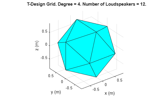
T-Design Loudspeaker Setup
You start your analysis with an (optimal) t-design loudspeaker setup. T-designs ensure that the loudspeakers are evenly distributed over the surface of a sphere, providing uniform coverage and accurate spatial audio reproduction.
Get the spherical coordinates of the t-design (in degrees).
loudspeakerSph = tdesignLoudspeakerLayout(Degree=4);
Plot the loudspeaker locations in space.
figure
tdesignLoudspeakerLayout(Degree=4)
The sampling ambisonic decoder (SAD) algorithm is optimal for t-designs [1]. Design a SAD decoding matrix. Assume an ambisonic order of 2.
order = 2;
D = ambisonicDecoderMatrix(order,loudspeakerSph,Decoder="sad");
In the next few sections, you explore metrics used to analyze the performance of the decoder with this loudspeaker setup.
Amplitude Range
Assume that the signal from a sound source coming from a certain direction is encoded into an ambisonic signal, and then decoded onto the loudspeakers. The amplitude, or coherent sum of the decoded signal is given by:
,
where is the decoded gain at the l-th loudspeaker.
A "good" decoder will yield a stable coherent sum at different source directions.
Derive the decoded amplitude for different source directions.
Start by creating a grid covering a range of azimuth and elevation ranges. Use an angular resolution of 5 degrees.
azimuthRange = [-180,180];
azimuthResolution = 5;
elevationRange = [-90 90];
elevationResolution = 5;

azimuthValues = azimuthRange(1):azimuthResolution:azimuthRange(2);
elevationValues = elevationRange(1):elevationResolution:elevationRange(2);
[azimuthGrid,elevationGrid] = meshgrid(azimuthValues, elevationValues);
sources = [azimuthGrid(:) elevationGrid(:)];

size(sources)
ans = 1×2

        2701           2
Create an ambisonic encoder matrix for all source directions.
E = ambisonicEncoderMatrix(order,sources);
Decode the sources.
Y = E*D;
size(Y)
ans = 1×2

        2701          12
Each row in Y holds the loudspeaker gains associated with one source direction.
Compute and normalize the decoded amplitude for every source direction.
P = sum(Y,2);
P = P./max(abs(P));
Compute the range of the amplitudes. Notice the range is tiny, which indicates that this decoder is performing well.
fprintf("Max amplitude: %f\n",max(P))Max amplitude: 1.000000
fprintf("Min amplitude: %f\n",min(P))Min amplitude: 1.000000
fprintf("Amplitude dynamic range: %f\n",max(P)-min(P))Amplitude dynamic range: 0.000000
Visualize the amplitude at different source directions. Include the locations of the loudspeakers in the plot for reference.
figure;
plotMetric(P, "Amplitude Range", azimuthValues,elevationValues,loudspeakerSph);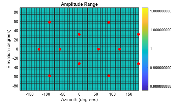
Energy Range
The energy metric is similar to the amplitude metric and is considered a superior criterion for evaluating decoders [2].
For a specific source direction, the energy is defined as:
.
A "good" decoder yields stable energy for all source directions.
Compute and normalize the decoded energy for every source direction.
E = sum(Y.^2,2);
ENorm = E./max(E);
Compute the range of the energy over all source directions.
fprintf("Max amplitude: %f\n",max(ENorm))Max amplitude: 1.000000
fprintf("Min amplitude: %f\n",min(ENorm))Min amplitude: 1.000000
fprintf("Amplitude dynamic range: %f\n",max(ENorm)-min(ENorm))Amplitude dynamic range: 0.000000
Visualize the amplitude at different source directions.
figure;
plotMetric(ENorm, "Energy Range", azimuthValues,elevationValues,loudspeakerSph);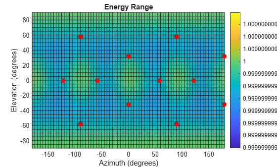
Velocity Vector Magnitude
The velocity vector is a popular metric for decoder accuracy at low frequencies [2].
The velocity vector is defined as:
,
where is the unit vector pointing to speaker l.
Convert the speaker spherical coordinates to cartesian coordinates.
[x,y,z] = sph2cart(loudspeakerSph(:,1)*pi/180,loudspeakerSph(:,2)*pi/180,1);
loudspeakerXYZ = [x,y,z];
Compute and normalize the magnitude of the velocity vector at all source directions.
rV = (Y*loudspeakerXYZ)./(P*ones(1,3));
rVMag = sqrt(sum(rV.^2,2));
rVMag = rVMag./max(rVMag);
Compute the range of the vector magnitude over all source directions.
fprintf("Max amplitude: %f\n",max(rVMag))Max amplitude: 1.000000
fprintf("Min amplitude: %f\n",min(rVMag))Min amplitude: 1.000000
fprintf("Amplitude dynamic range: %f\n",max(rVMag)-min(rVMag))Amplitude dynamic range: 0.000000
Visualize the velocity vector magnitude at different source directions.
figure;
plotMetric(rVMag, "Velocity Vector Magnitude", azimuthValues,elevationValues,loudspeakerSph);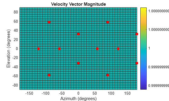
Velocity Vector Angular Error
The direction of the velocity vector must match the source direction.
The angular error between the source direction and the velocity vector direction is a popular quality metric at low frequencies [2].
Convert the source directions from spherical coordinates to cartesian coordinates.
sourceXYZ = zeros(size(sources,1),3);
[sourceXYZ(:,1),sourceXYZ(:,2),sourceXYZ(:,3)] = sph2cart(pi*sources(:,1)/180,pi*sources(:,2)/180,1);
Compute the angular error, in degrees.
U_rV = rV./(sqrt(sum(rV.^2,2))*ones(1,3));
dot_rV = sum(U_rV.*sourceXYZ,2);
dot_rV(dot_rV>1) = 1;
dot_rV(dot_rV<-1) = -1;
rVAng = acos(dot_rV)*180/pi;
Display the range of the velocity vector angular error over all source directions.
fprintf("Max angular error (degrees): %f\n",max(rVAng))Max angular error (degrees): 0.000001
fprintf("Min angular error (degrees): %f\n",min(rVAng))Min angular error (degrees): 0.000000
fprintf("Amplitude dynamic range (degrees): %f\n",max(rVAng)-min(rVAng))Amplitude dynamic range (degrees): 0.000001
Visualize the angular error at different source directions.
figure;
plotMetric(rVAng, "Velocity Vector Angular Error (Degrees)", azimuthValues,elevationValues,loudspeakerSph);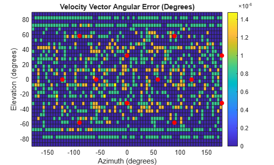
Energy Vector Magnitude
The energy vector is a better metric compared to the velocity vector at high frequencies [2].
The energy vector is defined as:
.
Compute and normalize the magnitude of the energy vector at all source directions.
rE = (Y.^2*loudspeakerXYZ)./(E*ones(1,3));
rEMag = sqrt(sum(rE.^2,2));
rEMagNorm = rEMag./max(rEMag);
Compute the range of the vector magnitude over all source directions.
fprintf("Max amplitude: %f\n",max(rEMagNorm))Max amplitude: 1.000000
fprintf("Min amplitude: %f\n",min(rEMagNorm))Min amplitude: 1.000000
fprintf("Amplitude dynamic range: %f\n",max(rEMagNorm)-min(rEMagNorm))Amplitude dynamic range: 0.000000
Visualize the energy vector magnitude at different source directions.
figure;
plotMetric(rEMagNorm, "Energy Vector Magnitude", azimuthValues,elevationValues,loudspeakerSph);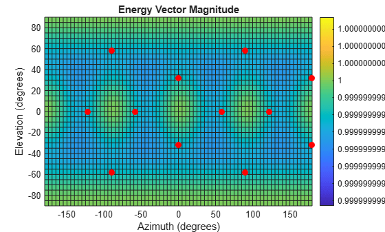
Energy Vector Angular Error
The energy vector angular error is preferred to the velocity vector error at high frequencies [2].
Compute the angular error, in degrees.
U_rE = rE./(sqrt(sum(rE.^2,2))*ones(1,3));
dot_rE = sum(U_rE.*sourceXYZ,2);
dot_rE(dot_rE>1) = 1;
dot_rE(dot_rE<-1) = -1;
rEAng = acos(dot_rE)*180/pi;
Compute the range of the velocity vector angular error over all source directions.
fprintf("Max angular error (degrees): %f\n",max(rEAng))Max angular error (degrees): 0.000001
fprintf("Min angular error (degrees): %f\n",min(rEAng))Min angular error (degrees): 0.000000
fprintf("Amplitude dynamic range (degrees): %f\n",max(rEAng)-min(rEAng))Amplitude dynamic range (degrees): 0.000001
Visualize the angular error at different source directions.
figure;
plotMetric(rEAng, "Velocity Vector Angular Error (Degrees)", azimuthValues,elevationValues,loudspeakerSph);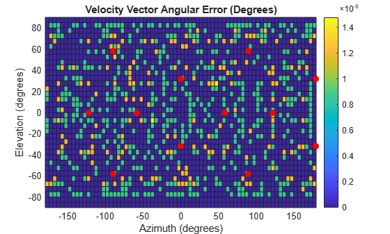
Apparent Source Width
Apparent source width (ASW) refers to the perceived spatial extent of a sound source. It quantifies how wide or narrow a sound appears to a listener.
The apparent source width is defined as (equation 2.11 in [1]):
.
Compute ASW for all source directions.
ASW = (5/8)*(180/pi)*2*acos(rEMag);
Compute the ASW range over all source directions.
fprintf("Max ASW (degrees): %f\n",max(ASW))Max ASW (degrees): 65.630938
fprintf("Min ASW (degrees): %f\n",min(ASW))Min ASW (degrees): 65.630938
fprintf("ASW dynamic range (degrees): %f\n",max(ASW)-min(ASW))ASW dynamic range (degrees): 0.000000
Visualize ASW for all source directions.
figure;
plotMetric(ASW, "ASW (Degrees)", azimuthValues,elevationValues,loudspeakerSph);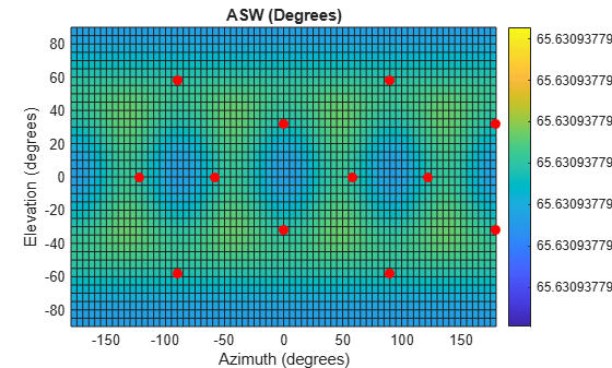
Dodecahedron Loudspeaker Setup
You have verified that the SAD decoder is optimal for a t-design loudspeaker setup.
Next, you verify the performance of the SAD decoder for a dodecahedron loudspeaker setup.
Define the loudspeaker locations.
loudspeakerSph = platonicSolidLoudspeakerLayout(Layout="dodecahedron");Design the ambisonic decoder for this loudspeaker setup. Assume an order of 3.
order = 3;
D = ambisonicDecoderMatrix(order, loudspeakerSph, Decoder="SAD");
In this section, you use the helper object ambisonicAnalyzer. The object encapsulates the metric computations from the previous section.
Define the ambisonic analyzer.
analyzer = ambisonicAnalyzer(Loudspeakers=loudspeakerSph,...
                             DecoderMatrix = D,...
                             AzimuthRange = [-180,180],...
                             AzimuthStep = 5,...
                             ElevationRange = [-90 90],...
                             ElevationStep = 5);
You can execute the following object methods to perform analysis similar to the previous section:
showLoudspeakers: Plot the loudspeaker setup.amplitudeRange: Analyze amplitude range.energyRange: Analyze energy range.velocityVectorMagnitude: Analyze the velocity vector magnitude.velocityVectorAngularError: Analyze the velocity vector angular error.energyVectorMagnitude: Analyze the energy vector magnitude.energyVectorAngularError: Analyze the energy vector angular error.apparentSourceWidth: Analyze ASW.
Analyze SAD
Show the non-uniform loudspeaker setup.
figure;
platonicSolidLoudspeakerLayout(Layout="dodecahedron");
View the energy vector magnitude for different source directions.
figure;
energyVectorMagnitude(analyzer)
Energy Vector Magnitude min: 0.919767
Energy Vector Magnitude max: 1.000000
Energy Vector Magnitude dynamic range: 0.080233

Notice that the vector magnitude shows higher variance with the source direction compared to the optimal t-design loudspeaker layout. The vector magnitude is maximized at the directions of the loudspeakers.
View the energy vector angular error for different source directions.
figure;
energyVectorAngularError(analyzer)
Energy Vector Angular Error min: 0.000000
Energy Vector Angular Error max: 4.393603
Energy Vector Angular Error dynamic range: 4.393603

Notice that the angular error is non-trivial for certain source directions. The angular error is minimized at the direction of the loudspeakers.
Analyze SAD with Max-RE Weighting
Max energy vector magnitude (Max-RE) weighting is often applied to ambisonic decoders to boost the magnitude of the energy vector [1], which is believed to reduce localization blur.
Compare the SAD decoder with max-RE weighting to the unweighted decoder for the same dodecahedron loudspeaker setup.
Design a SAD decoder with max-RE weighting.
D = ambisonicDecoderMatrix(order, loudspeakerSph, Decoder="SAD",ApplyMaxREWeighting=true);Create a new ambisonic analyzer for this decoder.
analyzerMaxRE = ambisonicAnalyzer(Loudspeakers=loudspeakerSph,...
                             DecoderMatrix = D,...
                             AzimuthRange = [-180,180],...
                             AzimuthStep = 5,...
                             ElevationRange = [-90 90],...
                             ElevationStep = 5);
Plot the energy vector magnitude for different source locations. Notice that the vector magnitude is boosted compared to the unweighted SAD case.
figure;
energyVectorMagnitude(analyzerMaxRE)
Energy Vector Magnitude min: 0.962782
Energy Vector Magnitude max: 1.000000
Energy Vector Magnitude dynamic range: 0.037218

Plot the energy vector angular error for different source locations. Notice that the error is reduced compared to the unweighted SAD case.
figure;
energyVectorAngularError(analyzerMaxRE)
Energy Vector Angular Error min: 0.000000
Energy Vector Angular Error max: 1.181464
Energy Vector Angular Error dynamic range: 1.181464

Irregular Loudspeaker Setup
Finally, consider an irregular loudspeaker setup.
loudspeakerSph = [45 -45 0 135 -135 15 -15 90 -90 180 45 -45  0 135 -135 90 -90 180  0  45 -45   0;
                  0   0 0   0    0  0   0  0   0   0 45  45 45  45   45 45  45  45 90 -30 -30 -30]';
Analyze SAD Decoder
Design the ambisonic decoder for this loudspeaker setup. Assume an order of 3.
order = 3;
D = ambisonicDecoderMatrix(order, loudspeakerSph, Decoder="SAD");
Define the ambisonic analyzer.
analyzerSAD = ambisonicAnalyzer(Loudspeakers=loudspeakerSph,...
                             DecoderMatrix = D,...
                             AzimuthRange = [-180,180],...
                             AzimuthStep = 5,...
                             ElevationRange = [-90 90],...
                             ElevationStep = 5);
View the loudspeaker setup.
figure;
showLoudspeakers(analyzerSAD)

Analyze the energy vector angular error.
figure
energyVectorAngularError(analyzerSAD)
Energy Vector Angular Error min: 0.349203
Energy Vector Angular Error max: 176.519964
Energy Vector Angular Error dynamic range: 176.170761

Analyze AllRAD Decoder
The All-Round Ambisonic Decoder (AllRAD) is an advanced decoder that combines SAD decoding with vector-base amplitude panning (VBAP). The AllRAD decoder can outperform the SAD decoder for irregular loudspeaker setups and yield lower directional error.
Create the AllRad decoder matrix.
D = ambisonicDecoderMatrix(order, loudspeakerSph, Decoder="allrad");Define the corresponding ambisonic analyzer.
analyzerAllRAD = ambisonicAnalyzer(Loudspeakers=loudspeakerSph,...
                             DecoderMatrix = D,...
                             AzimuthRange = [-180,180],...
                             AzimuthStep = 5,...
                             ElevationRange = [-90 90],...
                             ElevationStep = 5);
Analyze the energy vector angular error. Notice that is significantly reduced compared to the SAD decoder.
figure
energyVectorAngularError(analyzerAllRAD)
Energy Vector Angular Error min: 0.129477
Energy Vector Angular Error max: 26.561196
Energy Vector Angular Error dynamic range: 26.431719

Helper Functions
function plotMetric(metric, metricType, azimuthValues,elevationValues,Loudspeakers)
surf(azimuthValues, elevationValues, reshape(metric,numel(elevationValues),numel(azimuthValues)))
view(2)
colorbar
hold on
plot3(Loudspeakers(:,1), Loudspeakers(:,2), 2*max(metric(:))*ones(length(Loudspeakers),1), 'ro', 'MarkerFaceColor','r')
title(metricType)
xlabel("Azimuth (degrees)")
ylabel("Elevation (degrees)")
axis tight
end
References
[1] "All-Round Ambisonic Decoding: Spread and Correlation", F. Zotter et al, DAGA, 2022.
[2] "Optimized Decoders for Mixed-Order Ambisonics", A. Heller et al, Paper 10507, 150th Audio Engineering Society Convention, May 2021.
See Also
ambisonicEncoderMatrix | ambisonicDecoderMatrix