Compare Bluetooth LE Localization Techniques
R2026bThis example shows how to compare Bluetooth® low energy (LE) localization techniques by estimating the position of a stationary node from fixed locators. The example simulates received signal strength indicator (RSSI) based ranging, Bluetooth LE direction finding with angle of arrival (AoA) and angle of departure (AoD) techniques, and Bluetooth channel sounding (CS) with round-trip time (RTT) and phase-based ranging (PBR). It compares the position error for each method and shows how the errors vary with bit energy-to-noise density ratio (Eb/No).
In this example, you:
Configure a Bluetooth LE localization scenario with fixed locators and a stationary node in a two-dimensional (2-D) or three-dimensional (3-D) indoor environment.
Simulate five localization techniques of Bluetooth LE specifications: RSSI, AoA, AoD, RTT, and PBR.
Estimate the node position using lateration (range-based) and angulation (angle-based) architectures, and compute the Euclidean position error for each method.
Combine the PBR distance and AoA from a single locator to demonstrate the distance-angle technique.
Visualize the geometric range circles and rays for each localization method.
Characterize how each method degrades with noise by plotting average position error versus Eb/No.
Review Bluetooth LE Localization Measurements
Bluetooth Special Interest Group (SIG) [1] has progressively improved indoor positioning through successive specification releases. Each generation introduced a fundamentally different measurement type such as signal strength, signal direction, or signal timing.
RSSI
RSSI is the simplest and most widely deployed Bluetooth LE ranging technique. The system measures the received signal power (in dBm) and converts it to a distance estimate using a path-loss model. Because RSSI conflates propagation loss, ranging accuracy is typically limited to several meters. Despite this limitation, RSSI remains a practical baseline because it requires no specialized hardware. For more information on path-loss modeling, see bluetoothPathLoss.
Direction Finding (Bluetooth 5.1)
Bluetooth 5.1 introduced direction finding using constant tone extensions (CTEs). A transmitter appends an unmodulated carrier tone to the packet, and the receiver samples it across a switched antenna array to extract phase differences between elements. From these differences the system estimates the arrival or departure angle of the signal.
Two complementary techniques are defined by the SIG:
AoA technique— The receiving locator switches antennas across its antenna array while the transmitting node uses a single antenna. The locator estimates the azimuth (and, with a planar array, elevation) of the incoming signal. For more information, see .
AoD technique — The transmitting locator switches antennas across its antenna array while the receiving node uses a single antenna. The node estimates the departure angle from the locator, which by reciprocity gives the direction toward the locator. For more information, see .
An important limitation imposed by the SIG standard is that both the AoA and AoD techniques resolve angles within a half-wavelength array aperture, producing an inherent 180° front-back ambiguity. For a uniform linear array (ULA), the AoA technique estimates azimuth only. For a uniform rectangular array (URA), angle estimation extends to azimuth and elevation, but a ±90° field of view constraint still applies about the array in each dimension. Placing the field-of-view of each locator's array toward the room interior mitigates this limitation.
Channel Sounding (Bluetooth 6.3)
Bluetooth 6.0 introduced CS, a bidirectional procedure in which an initiator and a reflector exchange waveforms over multiple frequencies. This example uses two CS-based ranging techniques.
RTT measures the time it takes for a signal to travel from the initiator to the reflector and back. By using the signal propagation speed, the system estimates the distance as half the RTT multiplied by the speed of light, while accounting for processing delays. For more information on estimating the distance between Bluetooth LE devices by using RTT-based Channel Sounding, see Estimate Distance Between Bluetooth LE Devices by Using Channel Sounding and Round-Trip Timing.
PBR uses the phase difference of received signals across multiple frequencies to estimate distance. By transmitting signals at different frequencies and analyzing the resulting phase shifts, the system resolves ambiguities and achieves higher accuracy. For more information on estimating the distance between Bluetooth LE devices by using PBR-based Channel Sounding, see Estimate Distance Between Bluetooth LE Devices by Using Channel Sounding and Phase-Based Ranging.
Position Estimation
After collecting range or angle measurements from the locators, the example estimates the node position by using blePositionEstimate.
Lateration — RSSI, RTT, and PBR provide range estimates. The position estimator finds the point that best fits the range circles in 2-D or range spheres in 3-D. 2-D requires at least three nonlinear locators and 3-D requires at least four non-coplanar locators.
Angulation — The AoA and AoD techniques provide angle estimates. The position estimator finds the point that best fits the angle rays from the locators. At least two locators are required.
Distance-angle hybrid — One locator provides both a PBR range estimate and an AoA measurement. The position estimator combines the range and angle constraints from that locator.
Simulation Scenario
This example models an indoor Bluetooth LE localization scenario in a 2-D office environment. You can also run the example in a 3-D office environment. A set of fixed locators surrounds a stationary node at a known ground-truth position, as shown in this figure.
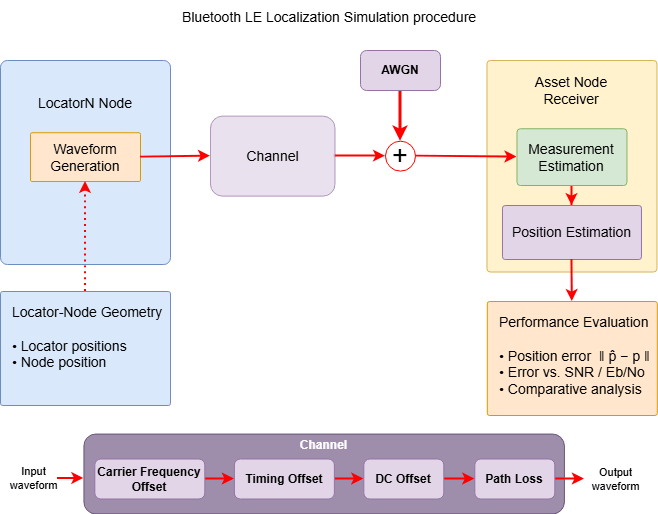
Overlapping coverage circles from multiple locators intersect near a central point, with dashed radial lines indicating range or angle measurements to estimated target positions in a 3-D coordinate space.
The scenario consists of:
Locators — Fixed Bluetooth LE devices at known positions that transmit or receive ranging waveforms
Node — The device whose position is estimated
Propagation model — Indoor path loss and additive white Gaussian noise (AWGN) at a configurable Eb/No
Each localization method operates independently on the same locator-node geometry. Lateration techniques estimate the distance from each locator to the node and solve for position from the range measurements. Angulation techniques estimate the angle from each locator to the node and solve for position from the rays.
Configure Simulation Parameters
To ensure repeatability, initialize the random number generator with the default seed. To improve statistical accuracy, you can run the simulation with different seeds and average the results across multiple runs.
rng("default");Configure Scenario Geometry
Set the number of spatial dimensions. For this example, set the value to 2 to use a planar 2-D scenario.
numDimensions =2; % 2 for 2-D, 3 for 3-D
Specify the simulation environment.
environmentModel =  "Office";
Set the localization techniques for analysis. For this example, select all of the available localization techniques: RSSI, AoA, AoD, RTT, and PBR.
localizationMethods = ["RSSI","AoA","AoD","RTT","PBR"];
Configure Waveform Parameter
Set the number of packets per locator and the Eb/No for the main simulation. Increasing the packet count improves estimate reliability by averaging over more observations. A higher Eb/No reduces the noise floor and sharpens ranging accuracy.
numPackets =20; EbNo =
24; sps = 8;
Set the number of iterations over which to average the position error.
numIterations =  20;
20;Set the data length.
dataLength =  200;
200;Create the Localization Simulator Object
Specify the PHY transmission mode as "LE1M" or "LE2M".
phyMode =  "LE2M";
Specify the duration of the CS tone as 10, 20, or 40 microseconds.
toneDuration =  40;
40;Specify the sounding sequence length as 32 or 96.
sequenceLength =  96;
96;Configure the antenna array and element spacing based on the number of spatial dimensions. The array size must be scalar representing ULA which supports azimuth estimation in the 2-D scenario. A vector array size representing URA which supports azimuth and elevation estimation in the 3-D scenario. Element spacing represents normalized spacing between the antenna elements with respect to wavelength.
arraySize =4; elementSpacing =
0.5;
Specify the direction finding packet type.
dfPacketType ="ConnectionCTE"; % Direction finding packet type
Set the element spacing as scalar for 2-D and a vector for 3-D scenario.
if numDimensions == 3 && isscalar(elementSpacing)
    elementSpacing = [elementSpacing elementSpacing];
end
Specify the slot duration and CTE length in microseconds.
slotDuration =2; cteLength =
160; % In the range [16, 160] with 8 microseconds step size
Validate the array size.
if numDimensions == 2 && size(arraySize,2) ~= 1
    error('The arraySize must be a scalar for 2-D position estimation');
end
if numDimensions == 3 && size(arraySize,2) ~= 2
    error('The arraySize must be a 1-by-2 vector for 3-D position estimation');
end
Create the localization simulator object by using helperBLELocalizationSimulator.
simulator = helperBLELocalizationSimulator(Mode=phyMode, ...
    SamplesPerSymbol=sps, ...
    Environment=environmentModel, ...
    DataLength=dataLength, ...
    SequenceLength=sequenceLength, ...
    ToneDuration=toneDuration, ...
    CTELength=cteLength, ...
    SlotDuration=slotDuration, ...
    DFPacketType=dfPacketType, ...
    CRCInit='555551', ...
    Iterations=numIterations, ...
    ArraySize=arraySize, ...
    ElementSpacing=elementSpacing, ...
    NumPackets=numPackets, ...
    LocalizationMethods=localizationMethods);
Place Locators and Node
Compute the locator positions and node position for the selected dimensionalities.
[posLocators,posNode,distance,angle] = getGeometry(simulator,numDimensions);
numLocators = size(posLocators,2);
numMethods = numel(localizationMethods);
Set the signal-to-noise ratio (SNR).
snr = EbNo - 10*log10(simulator.SamplesPerSymbol);
fprintf("Running %d-D simulation with %d locators, %d packets per locator, Eb/No = %d dB.\n", ...
    numDimensions,numLocators,numPackets,EbNo);
Running 2-D simulation with 3 locators, 20 packets per locator, Eb/No = 24 dB.
Simulate and Visualize
Simulate the selected Bluetooth LE localization methods across the deployed locator set. For each method, the step function transmits waveforms, applies indoor path loss, RF impairments, and AWGN, and estimates either range or angle measurements from the locators. The function then estimates the node position by using blePositionEstimate.
[distResults,angResults,posEstimates,posErrors,methodTimes] = ...
    step(simulator,posLocators,posNode,distance,angle,snr);
Display the position error and simulation time for each method.
for mIdx = 1:numMethods
    fprintf(" Method %4s: Position error = %2.2f meters, Simulation time = %1.3f seconds.\n", ...
        localizationMethods(mIdx),posErrors(mIdx),methodTimes(mIdx));
end
 Method RSSI: Position error = 2.50 meters, Simulation time = 1.005 seconds.
 Method  AoA: Position error = 0.01 meters, Simulation time = 0.927 seconds.
 Method  AoD: Position error = 0.02 meters, Simulation time = 0.649 seconds.
 Method  RTT: Position error = 0.09 meters, Simulation time = 1.225 seconds.
 Method  PBR: Position error = 0.16 meters, Simulation time = 0.549 seconds.
Compute Hybrid Distance-Angle Estimate
Combine the PBR range estimate with the AoA measurement from the closest locator to demonstrate a range-angle hybrid estimate. Under the path-loss and AWGN assumptions in this simulation, the closest locator typically provides the strongest received signal. The example solves the position by using the "distance-angle" mode of blePositionEstimate.
pbrIdx = find(localizationMethods == "PBR");
aoaIdx = find(localizationMethods == "AoA");
includeHybrid = ~isempty(pbrIdx) && ~isempty(aoaIdx);
if includeHybrid
    [~,closestIdx] = min(distance);
    hybridRange = distResults(pbrIdx,closestIdx);
    hybridAngle = angResults(1,aoaIdx,closestIdx);
    if numDimensions == 3
        hybridAngle = [hybridAngle;angResults(2,aoaIdx,closestIdx)];
    end
    estHybrid = blePositionEstimate(posLocators(:,closestIdx),"distance-angle",hybridRange,hybridAngle);
    errorHybrid = norm(estHybrid - posNode);
end
Organize the results by measurement architecture. RSSI, RTT, and PBR use range-based lateration. The AoA and AoD techniques use angle-based angulation. The hybrid row combines one PBR range estimate and one AoA angle estimate.
canonicalMethods = ["RSSI","AoA","AoD","RTT","PBR"];
canonicalArchLabels = ["Lateration","Angulation","Angulation","Lateration","Lateration"];
[~, archIdx] = ismember(localizationMethods,canonicalMethods);
architectureLabels = canonicalArchLabels(archIdx);
methodColumn = localizationMethods(:);
archColumn = architectureLabels(:);
errorColumn = posErrors(:);
timeColumn = methodTimes(:);
if includeHybrid
    methodColumn = [methodColumn;"Hybrid"];
    archColumn = [archColumn;"Distance-Angle"];
    errorColumn = [errorColumn;errorHybrid];
    timeColumn = [timeColumn;timeColumn(pbrIdx)+timeColumn(aoaIdx)];
end
resultsTable = table( ...
    methodColumn,archColumn,errorColumn,timeColumn, ...
    'VariableNames',{'Method','Architecture','Error (meters)','Time (seconds)'});
disp(resultsTable)
     Method       Architecture      Error (meters)    Time (seconds)
    ________    ________________    ______________    ______________

    "RSSI"      "Lateration"             2.4951           1.0048
    "AoA"       "Angulation"           0.014909          0.92659
    "AoD"       "Angulation"           0.019056            0.649
    "RTT"       "Lateration"           0.089057           1.2246
    "PBR"       "Lateration"             0.1554          0.54915
    "Hybrid"    "Distance-Angle"       0.063064           1.4757
Compute the average position error across the simulated methods.
fprintf("\nAverage position error across all methods: %.3f m, Eb/No: %d dB.\n", ...
    mean(posErrors), EbNo);
Average position error across all methods: 0.555 m, Eb/No: 24 dB.
Plot the geometric constraints imposed on the node position by each localization method.
visualizeLocalization(simulator,posLocators,posNode,distResults,angResults, ...
    posEstimates,posErrors,numDimensions,localizationMethods);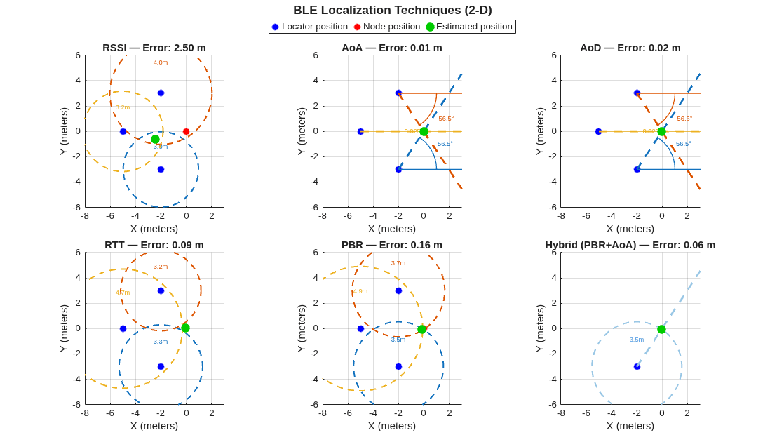
RSSI circles intersect over a broad area because the path-loss model maps signal strength to distance with large uncertainty. RTT and PBR circles tighten near the true node, while AoA and AoD rays converge close to it. The hybrid panel solves the position from a single locator's range and angle, showing how combining both angle and range constraints enables you to localize from a single anchor.
Analyze Error Across Eb/No
Evaluate how position error varies with Eb/No. Each point reports the mean position error over the simulation trials used by the helper object at that Eb/No value.
EbNoVector = 18:3:30;  % Eb/No values, in dB
simulator.NumPackets = [10 10 10 50 50];
Convert Eb/No values to SNR values.
snrVector = EbNoVector-10*log10(sps);
numSnr = numel(EbNoVector);
avgError = zeros(numMethods,numSnr);
Run the simulation at each Eb/No value.
for countSnr = 1:numSnr
    [~,~,~,avgError(:, countSnr)] = step(simulator,posLocators,posNode,distance,angle,snrVector(countSnr));
end
Display the average position error for each method.
disp("Average position error (meters) for each Bluetooth LE localization method")Average position error (meters) for each Bluetooth LE localization method
disp(array2table(avgError,'VariableNames',EbNoVector+" dB",'RowNames',localizationMethods))
             18 dB        21 dB       24 dB       27 dB       30 dB
            ________    _________    ________    ________    ________

    RSSI     0.79801      0.80972     0.81739     0.82172     0.82399
    AoA     0.010212    0.0098518    0.011171    0.011911    0.012148
    AoD     0.014017     0.013291    0.013574    0.014149    0.013753
    RTT      0.42916      0.33145     0.27673     0.24806     0.21918
    PBR      0.12378      0.15026    0.084041    0.071396    0.023011
Plot the average position error against Eb/No for each localization technique.
plotResults(simulator,avgError,EbNoVector,localizationMethods);
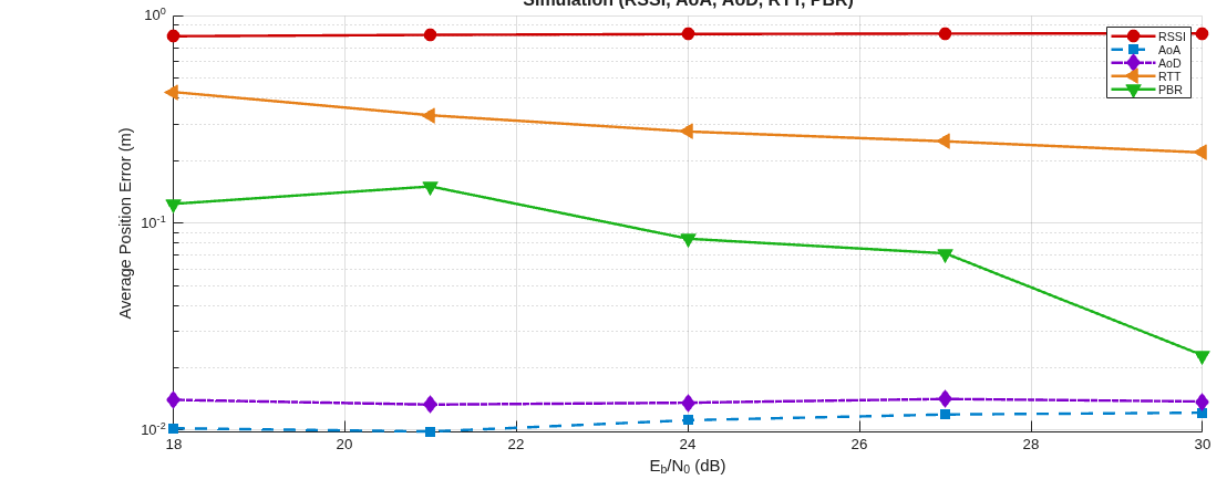
This plot shows how average position error varies with Eb/No for each method. Each point represents the average error across the fixed locator-node geometry at each Eb/No value. The performance of the RSSI curve is poor, confirming that its accuracy is bounded by path-loss model uncertainty rather than Eb/No. The AoA and AoD techniques improve gradually as the antenna-array phase estimates become less noisy. The RTT and PBR curves drop the fastest, illustrating the submeter ranging precision that Channel Sounding delivers once Eb/No is high enough to resolve the timing/phase measurements reliably.
Appendix
The example uses these helper functions.
helperBLEGenerateDFPDU.m— Generate direction finding packet PDUhelperBLEImpairmentsAddition.m— Add RF impairments to the Bluetooth LE waveformhelperBLEImpairmentsInit.m— Initialize RF impairment parametershelperBLELocalizationSimulator.m— Simulate the selected Bluetooth LE localization methods, estimate node position, and provide visualization utilities.helperBLEPhaseEstimate.m— Estimate phase rotations from the Bluetooth LE CS tone waveform.helperBLESteeringVector.m— Generate steering vectorhelperBLESteerSwitchAntenna.m— Perform antenna steering and switchinghelperBLESwitchAntenna.m— Perform antenna switchinghelperBLETOAEstimate.m— Estimate time of arrival from the Bluetooth LE CS SYNC waveform.helperBLEVisualizePosition.m— Visualize localization geometry and constraints.
References
[1] Bluetooth Technology Website. "Bluetooth Technology Website | The Official Website of Bluetooth Technology." Accessed May 22, 2026. https://www.bluetooth.com/.
[2] Bluetooth Core Specifications Working Group. "Bluetooth Core Specification" v6.3. https://www.bluetooth.com/specifications/specs/core-specification-6-3/.
[3] Bluetooth Range Estimator. "Path Loss (Propagation) Models." Bluetooth Special Interest Group (SIG). https://www.bluetooth.com.
See Also
Functions
bleWaveformGenerator|bleAngleEstimate|blePositionEstimate|bluetoothRange|bleWaveformGenerator
Objects
Topics
- What Is Bluetooth Channel Sounding?
- Estimate Distance Between Bluetooth LE Devices by Using Channel Sounding and Round-Trip Timing
- Estimate Distance Between Bluetooth LE Devices by Using Channel Sounding and Phase-Based Ranging
- Estimate Bluetooth LE Node Position
- Bluetooth Location and Direction Finding
- Bluetooth LE Direction Finding for Tracking Node Position
- Bluetooth LE Positioning with Deep Learning

