comm.AGC
Adaptively adjust gain for constant signal level output
Description
The comm.AGC
System object™ creates an automatic gain controller (AGC) that adaptively adjusts its
gain to achieve a constant signal level at the output. For more information, see Logarithmic-Loop AGC.
This object is designed for streaming applications. For more information, see Tips.
To adaptively adjust gain for a constant signal level at the output:
Create the
comm.AGCobject and set its properties.Call the object with arguments, as if it were a function.
To learn more about how System objects work, see What Are System Objects?
Creation
Description
agc = comm.AGC
agc = comm.AGC(Name,Value)AdaptationStepSize',0.05 sets the step size
for gain updates to 0.05.
Properties
Usage
Description
Y = agc(X)
[
returns Y,powerlevel] = agc(X)powerlevel, the power level estimate of the input
signal. You can use powerlevel as an energy detector
output.
Input Arguments
Output Arguments
Object Functions
To use an object function, specify the
System object as the first input argument. For
example, to release system resources of a System object named obj, use
this syntax:
release(obj)
Examples
Apply different AGC averaging lengths to QAM-modulated signals. Compare the variance and plot of the signals after AGC is applied.
Create three AGC System objects with their average window lengths set to 10, 100, and 1000 samples, respectively.
agc1 = comm.AGC('AveragingLength',10);
agc2 = comm.AGC('AveragingLength',100);
agc3 = comm.AGC('AveragingLength',1000);
Generate 16-QAM modulated and raised cosine pulse shaped packetized data.
M = 16;
d = randi([0 M-1],1000,1);
s = qammod(d,M);
x = 0.1*s;
pulseShaper = comm.RaisedCosineTransmitFilter;
y = awgn(pulseShaper(x),inf);
Apply AGC to the data capturing separate outputs for each AGC object.
r1 = agc1(y);
r2 = agc2(y);
r3 = agc3(y);
Plot and compare the signals. As the averaging length increases, the variance at the output of AGC decreases.
figure(1)
subplot(4,1,1)
plot(abs(y))
title('AGC Input')
subplot(4,1,2)
plot(abs(r1))
axis([0 8000 0 10])
title('AGC Output (Averaging Length is 10 Samples)')
text(4000,5,sprintf('Variance is %f',var(r1(3000:end))))
subplot(4,1,3)
plot(abs(r2))
axis([0 8000 0 10])
title('AGC Output (Averaging Length is 100 Samples)')
text(4000,5,sprintf('Variance is %f',var(r2(3000:end))))
subplot(4,1,4)
plot(abs(r3))
axis([0 8000 0 10])
title('AGC Output (Averaging Length is 1000 Samples)')
text(4000,5,sprintf('Variance is %f',var(r3(3000:end))))

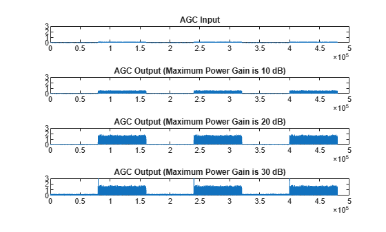
Apply different AGC maximum gain levels to QPSK-modulated signals. Compare the plot of the signals after AGC is applied.
Create three AGC System objects with their maximum gain values set to 10, 20, and 30 dB, respectively.
agc1 = comm.AGC('MaxPowerGain',10);
agc2 = comm.AGC('MaxPowerGain',20);
agc3 = comm.AGC('MaxPowerGain',30);
Generate QPSK-modulated data. Pass the data through raised cosine pulse shaped filtering and an AWGN channel.
M = 4;
pktLen = 10000;
d = randi([0 M-1],pktLen,1);
s = pskmod(d,M,pi/4);
x = repmat([zeros(pktLen,1); 0.3*s],3,1);
pulseShaper = comm.RaisedCosineTransmitFilter;
y = awgn(pulseShaper(x),50);
Apply AGC to the data capturing separate outputs for each AGC object.
r1 = agc1(y);
r2 = agc2(y);
r3 = agc3(y);
Plot the input signal and the AGC-adjusted signal with various maximum gain levels. Compare the results for the conditions in this example.
A maximum gain setting of 10 dB is too small, and the AGC output does not reach the desired output signal level risking data loss due to decreased signal dynamic range.
A maximum gain setting of 20 dB is optimal, and the AGC output reaches the desired level without signal loss due to saturation.
A maximum gain setting of 30 dB is too large, and the AGC output overshoots the desired signal level risking signal saturation and data loss at the start of received packets.
Between packets the input signal contains only noise.
As shown in the plots, the packet transmissions have extended periods when no data is received. The extended periods with no data received results in AGC increasing to the maximum gain setting. If a packet arrives when the AGC gain is too high, the output power overshoots the desired signal level until the AGC can respond to the change in the input power level and reduce its gain.
limits = [0 3];
figure(1)
subplot(4,1,1)
plot(abs(y))
ylim(limits)
title('AGC Input')
subplot(4,1,2)
plot(abs(r1))
ylim(limits)
title('AGC Output (Maximum Power Gain is 10 dB)')
subplot(4,1,3)
plot(abs(r2))
ylim(limits)
title('AGC Output (Maximum Power Gain is 20 dB)')
subplot(4,1,4)
plot(abs(r3))
ylim(limits)
title('AGC Output (Maximum Power Gain is 30 dB)')
Plot a signal and the power level estimate. Compare the results. The power level estimate can serve as a power detector, indicating exactly when the received packet has arrived.
Create an AGC System object with its maximum gain value set to 20 dB.
agc20 = comm.AGC('MaxPowerGain',20);Generate QPSK-modulated data. Pass the data through raised cosine pulse shaped filtering and an AWGN channel.
modOrd = 4; % Modulation order
pktLen = 10000; % Packet length
d = randi([0 modOrd-1],pktLen,1);
s = pskmod(d,modOrd,pi/4);
x = repmat([zeros(pktLen,1); 0.3*s],3,1);
pulseShaper = comm.RaisedCosineTransmitFilter;
y = awgn(pulseShaper(x),50);
Apply AGC to the data capturing separate outputs for each AGC object.
[r2,p2] = agc20(y);
Plot the input signal and the received signal power level estimate. Compare the results. Reception of packetized data with extended periods when no data is received results in the detected power level estimate decreasing to nearly zero. While an input signal is detected, the output power level estimate, p2, serves as a power detector, indicating exactly when the received packet has arrived.
limits = [0 3];
figure(1)
subplot(4,1,1)
plot(abs(y))
ylim(limits)
title('AGC Input')
subplot(4,1,2)
plot(abs(p2))
title('Power Level')

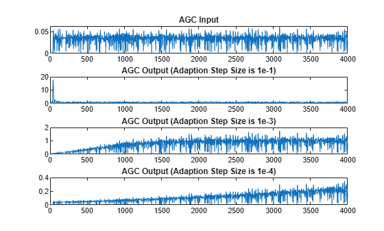
Apply different AGC step sizes to QPSK-modulated signals. Compare the signals after applying AGC.
Create three AGC System objects with their step sizes set to 1e-1, 1e-3, and 1e-4, respectively.
agc1 = comm.AGC('AdaptationStepSize',1e-1);
agc2 = comm.AGC('AdaptationStepSize',1e-3);
agc3 = comm.AGC('AdaptationStepSize',1e-4);
Generate QPSK-modulated data with raised cosine pulse shaping.
d = randi([0 3],500,1);
s = pskmod(d,4,pi/4);
x = 0.1*s;
pulseShaper = comm.RaisedCosineTransmitFilter;
y = pulseShaper(x);
Apply AGC to the data capturing separate outputs for each AGC object.
r1 = agc1(y);
r2 = agc2(y);
r3 = agc3(y);
Plot the input and output signal after the various AGC step sizes.
With the step size set to 1e-1, the AGC output signal overshoot is evident. The output signal converges very quickly.
With the step size set to 1e-3, the AGC output signal overshoot disappears. The output signal gradually converges.
With the step size set to 1e-4, the AGC output signal takes 2 to 3 times longer to converge than a step size of 1e-3.
figure
subplot(4,1,1)
plot(abs(y))
title('AGC Input')
subplot(4,1,2)
plot(abs(r1))
title('AGC Output (Adaption Step Size is 1e-1)')
subplot(4,1,3)
plot(abs(r2))
title('AGC Output (Adaption Step Size is 1e-3)')
subplot(4,1,4)
plot(abs(r3))
title('AGC Output (Adaption Step Size is 1e-4)')
Modulate and amplify a QPSK signal. Set the received signal amplitude to approximately 1 volt by using an AGC. Plot the output.
Create a QPSK-modulated signal by using the QPSK System object.
data = randi([0 3],1000,1);
modData = pskmod(data,4,pi/4);
Attenuate the modulated signal.
txSig = 0.1*modData;
Create an AGC System object and pass the transmitted signal through it. The AGC adjusts the received signal power to approximately 1 W.
agc = comm.AGC;
rxSig = agc(txSig);
Plot the signal constellations of the transmit and received signals after the AGC reaches steady-state.
h = scatterplot(txSig(200:end),1,0,'*');
hold on
scatterplot(rxSig(200:end),1,0,'or',h);
legend('Input of AGC','Output of AGC')
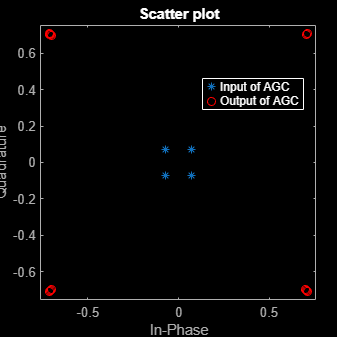
Measure and compare the power of the transmitted and received signals after the AGC reaches a steady state. The power of the transmitted signal is 100 times smaller than the power of the received signal.
txPower = var(txSig(200:end));
rxPower = var(rxSig(200:end));
[txPower rxPower]
ans = 1×2

    0.0100    0.9970
Create two AGC System objects™ to adjust the level of the received signal using two different step sizes with identical update periods.
Generate an 8-PSK signal such that its power is 10 W.
data = randi([0 7],200,1);
modData = sqrt(10)*pskmod(data,8,pi/8,'gray');
Create a pair of raised cosine matched filters with their Gain property set so that they have unity output power.
txfilter = comm.RaisedCosineTransmitFilter('Gain',sqrt(8));
rxfilter = comm.RaisedCosineReceiveFilter('Gain',sqrt(1/8));
Filter the modulated signal through the raised cosine transmit filter.
txSig = txfilter(modData);
Create two AGC System objects to adjust the received signal level. Set a step size of 0.01 and 0.1, respectively.
agc1 = comm.AGC('AdaptationStepSize',0.01);
agc2 = comm.AGC('AdaptationStepSize',0.1);
Apply AGC to the modulated signal capturing separate outputs for each AGC object.
agcOut1 = agc1(txSig);
agcOut2 = agc2(txSig);
Filter the AGC output signals by using the raised cosine receive filter.
rxSig1 = rxfilter(agcOut1);
rxSig2 = rxfilter(agcOut2);
Plot the power of the filtered AGC responses while accounting for the 10 symbol delay through the transmit-receive filter pair.
plot([abs(rxSig1(11:110)).^2 abs(rxSig2(11:110)).^2])
grid on
xlabel('Symbols')
ylabel('Power (W)')
legend('Step size 0.01','Step size 0.1')
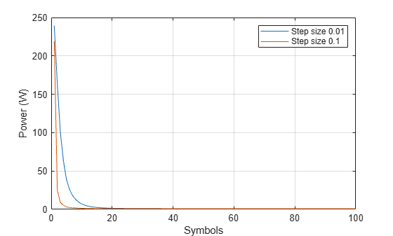
The signal with the larger step size converges faster to the AGC target power level of 1 W.
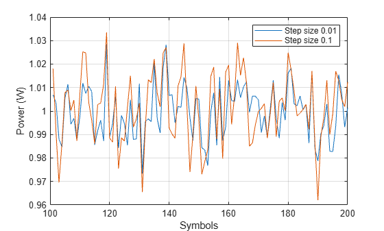
Plot the power of the steady-state filtered AGC signals by including only the last 100 symbols. The larger AGC step size results in less accurate gain correction. Larger AGC step size values result in faster convergence at the expense of less accurate gain control.
plot((101:200),[abs(rxSig1(101:200)).^2 abs(rxSig2(101:200)).^2])
grid on
xlabel('Symbols')
ylabel('Power (W)')
legend('Step size 0.01','Step size 0.1')
Pass attenuated QPSK packet data to two AGCs with different maximum gains. Plot the results.
Create two, 200-symbol QPSK data packets. Transmit the packets over a 1200-symbol frame.
modData1 = pskmod(randi([0 3],200,1),4,pi/4);
modData2 = pskmod(randi([0 3],200,1),4,pi/4);
txSig = [modData1; zeros(400,1); modData2; zeros(400,1)];
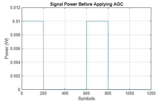
Attenuate the transmitted burst signal by 20 dB and plot its power.
rxSig = 0.1*txSig;
rxSigPwr = abs(rxSig).^2;
plot(rxSigPwr)
grid
xlabel('Symbols')
ylabel('Power (W)')
title('Signal Power Before Applying AGC')
Create two AGCs with maximum power gains of 30 dB and 24 dB, respectively.
agc1 = comm.AGC('MaxPowerGain',30,'AdaptationStepSize',0.02);

agc2 = comm.AGC('MaxPowerGain',24,'AdaptationStepSize',0.02);
Apply AGC to the attenuated signal capturing separate outputs for each AGC object. Calculate the output power for each case.
rxAGC1 = agc1(rxSig);
rxAGC2 = agc2(rxSig);

pwrAGC1 = abs(rxAGC1).^2;
pwrAGC2 = abs(rxAGC2).^2;
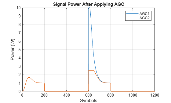
Plot the output powers. Initially, for the second packet, the agc1 output signal power is too high because the AGC applied its maximum gain during the period when no data was transmitted. The corresponding agc2 output signal power (2.5 W) overshoots the target power level of 1 W by significantly less than the agc1 output signal power (10 W). The convergence time for agc2 is shorter than the convergence time for agc1, because the signal input to agc2 applies a smaller maximum gain than agc1.
plot([pwrAGC1 pwrAGC2])
legend('AGC1','AGC2')
grid
xlabel('Symbols')
ylabel('Power (W)')
title('Signal Power After Applying AGC')
More About
The AGC implementation uses a logarithmic feedback loop. As this figure of the logarithmic-loop AGC algorithm shows, the output signal is the product of the input signal and the exponential of the loop gain. The error signal is the difference between the reference level and the product of the logarithm of the detector output and the exponential of the loop gain. After multiplying by the step size, the AGC passes the error signal to an integrator.

The logarithmic-loop AGC performs well for a variety of signal types, including amplitude modulation. The AGC Detector is applied to the input signal, which improves convergence times, but increases signal power variation at the detector input. Large signal variation at the detector input is acceptable for floating-point systems.
Mathematically, the algorithm is summarized as
where:
x is the input signal.
y is the output signal.
g is the loop gain.
Detector(•) is the detector function.
z is the detector output.
A is the reference value.
err is the error signal.
K is the step size.
Tips
This System object is designed for streaming applications.
If the signal amplitude does not change within the frame, you can simulate an ideal AGC by calculating the average gain desired for a frame of samples. Then, apply the gain to each sample in the frame.
If you use the AGC with higher order QAM signals, you might need to reduce the variation in the gain during steady-state operation. Inspect the constellation diagram at the output of the AGC during steady-state operation. You can increase the averaging length to avoid frequent gain adjustments. An increase in averaging length reduces execution speed.