timingEstimate
Syntax
Description
Examples
Generate a QPSK reference signal and input waveform. Fix the random seed.
 s = rng(123);
refSignal = pskmod(randi([0 3],[512 1]),4,pi/4);
waveform = pskmod(randi([0 3],[512 1]),4,pi/4);
Check the timing offset by using the reference signal as both inputs. Expected offset is 0.
offset1 = timingEstimate(refSignal,refSignal)
offset1 =
0
Check the timing offset between the input waveform and the reference signal.
offset2 = timingEstimate(waveform,refSignal) % Expected offset is []offset2 =
[]
offset3 = timingEstimate([zeros(5,1);refSignal],refSignal) % Expected offset is 5offset3 = 5
offset4 = timingEstimate([refSignal(2:end);0],refSignal) % Expected offset is -1offset4 = -1
Generate a noise waveform input to compare with the reference signal.
noisyWaveform = awgn(refSignal,-15,'measured');Estimate the timing offset and the normalized correlation magnitude between the noisy waveform and the reference signal.
[offset5, normCorr] = timingEstimate(noisyWaveform,refSignal) % Expected offset is []offset5 =
[]
normCorr = 1023×1

    0.0442
    0.0198
    0.0066
    0.0462
    0.0556
    0.0391
    0.0425
    0.0149
    0.0185
    0.0532
    0.0680
    0.0080
    0.0284
    0.0642
    0.0193
      ⋮
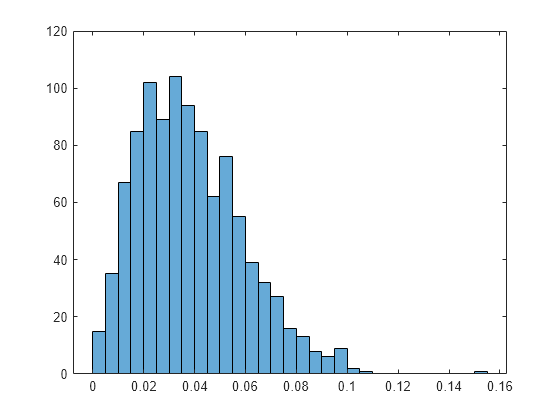
Adjust the threshold to control the probability of missed detection. If needed, collect more normalized correlation data.
histogram(normCorr(:))

offset6 = timingEstimate(noisyWaveform,refSignal,Threshold=0.05) % Expected offset is 0offset6 = 0
Restore random seed.
rng(s);
Adjust the window length for a timing offset estimate to reduce intersymbol interference (ISI) in orthogonal frequency division multiplexing (OFDM) transmission.
Specify the OFDM parameters.
nfft = 512;
cplen = 16;
symLen = nfft + cplen;
nullIdx = [1:6 nfft/2+1 nfft-5:nfft]';
numDataCarrs = nfft-length(nullIdx);
modOrder = 64;
Generate the OFDM signal. Fix the random seed.
s = rng(123);
numSym = 100;
srcBits = randi([0,1], [numDataCarrs*log2(modOrder) numSym+2]);
ofdmData = qammod(srcBits,modOrder,InputType='bit', ...
            UnitAveragePower=true);
txSignal = ofdmmod(ofdmData,nfft,cplen,nullIdx);
Use the second OFDM symbol as a reference signal.
refSig = txSignal(symLen+(1:symLen));
Generate a channel filter randomly. Make h(4) the biggest peak.
h = 10*randn(cplen+1,1,'like',1j);
h(4) = h(4)/abs(h(4))*(2*max(abs(h)));
Pass reference signal through a filter. Add delay and noise.
rxSignal = awgn([zeros(213,1);filter(h,1,txSignal)], ...
           70,"measured");
With the WindowLength property equal to the default value, the estimated timing offset points to the largest peak in the channel impulse response. But just using the default value for window length may not provide the timing offset required for reducing ISI. With the WindowLength=cplen+1, the function focuses on a window that is the length of the cyclic prefix (cplen) plus one sample. Then estimated timing offset shifts as much energy of the channel impulse response as possible into the cyclic prefix region of an OFDM symbol, aligning the timing offset with the received signal and reducing the ISI.
windowLenVec = [1 (cplen+1)];
 for k = 1:length(windowLenVec)
    % Get timing estimate
    offset = timingEstimate(rxSignal,refSig,WindowLength=windowLenVec(k));
    % Demodulate signal
    rxofdmData = ofdmdemod(rxSignal(offset+(1:symLen*numSym)), ...
                 nfft,cplen,cplen,nullIdx).';
    % Find the best possible equalizer by using
    % known data
    equalizerCoef = zeros(numDataCarrs,1);
     for n = 1:numDataCarrs
         equalizerCoef(n) = rxofdmData(:,n)\(ofdmData(n,1+(1:numSym)).');
     end
    % Equalize signal
    eqData = rxofdmData*diag(equalizerCoef);
    % Plot constellation diagram for all subcarriers
    % Set WindowLength=cplen+1 leads to a timing estimate that reduces ISI
    constdiag{k} = comm.ConstellationDiagram(ShowReferenceConstellation=false);
    constdiag{k}.Title = ['WindowLength = ' num2str(windowLenVec(k))...
                          ', Offset = ' num2str(offset)];
    constdiag{k}(eqData(:));
  end


Restore the random seed.
rng(s);
Input Arguments
Input waveform, specified as a T-by-Nr matrix where:
T is the number of time domain samples.
Nr is the number of receive antennas.
Note
For GPU processing, both waveform and
refsig inputs must be a gpuArray
object.
Data Types: double | single
Reference signal, specified as an L-by-Nt matrix where:
L is the number of time domain samples.
Nt is the number of transmit streams.
Note
For GPU processing, both waveform and
refsig inputs must be a gpuArray
object.
Data Types: double | single
Name-Value Arguments
Specify optional pairs of arguments as
Name1=Value1,...,NameN=ValueN, where Name is
the argument name and Value is the corresponding value.
Name-value arguments must appear after other arguments, but the order of the
pairs does not matter.
Example: Z = timingEstimate(Y,M,Threshold=0.2);
Detection threshold, specified as a real scalar between 0 and 1. If any normalized cross-correlation magnitude is equal to or greater than this threshold, the function decides that the reference signal is in the waveform.
Data Types: single | double
Window length of consecutive samples, specified as a positive integer.
Data Types: single | double
Output Arguments
Estimated timing offset, returned as an integer, given by an integer number of samples relative to the first sample of the input waveform.
If the
offsetis nonnegative,waveform(offset+(1:L),:)is a good match to the reference signal.If
offsetis negative, the receivedwaveformis late late.waveform(1:(L+offset),:)is a good match torefsig(1-offset:L,:).If
waveformis not a good match torefsig,offsetis an empty array.
Normalized correlation magnitude, returned as a (T+L-1)-by-Nr-by-Nt array. Each element in the array is a real value in the range [0,1]. A larger value indicates a stronger correlation between the input waveform and the reference signal for the corresponding offset, receive antenna, and the transmit stream.
If all values in
normcorrare less than the default threshold of 0.2, the function returns an empty array foroffset.If
normcorrmeets or exceeds the default threshold value, the function calculatesoffsetfrom theNt*Nrestimated channel impulse responses between the transmit streams and the receive antennas.
Algorithms
The timing offset indicates the estimated location of a reference signal in the received
signal, if the reference signal is present in the received signal. The
timingEstimate function helps to calculate this offset. This
function has two key stages. The first stage decides whether the reference signal is in the
received waveform. If the reference signal is in the received waveform, then the second
stage estimates the timing offset.
Both algorithms the function uses are based on cross-correlating the reference signal and the received waveform.
The detection algorithm uses the principle of a matched filter or cross-correlator to detect the presence and location of a reference signal within a received waveform. In cross-correlation, you slide a reference or given signal across a received signal and calculate the similarity between the signal. If you plot this on a graph, the peaks in the cross-correlated signal indicate potential locations of the reference signal within the received signal at a particular time. The higher the peak the more the similarity between the reference signal and the received signal. Several factors influence the magnitude of the cross-correlation peaks. These factors could be the energy of the reference signal, the energy of the received signal, and the noise level, to name a few. You can normalize or scale the peaks for a more accurate detection of the given signal. Without appropriate scaling, it becomes harder to compare the correlation peaks, which makes the detection more difficult or inaccurate.
Consider this:
refSignal = 2.3*randn(256,1,'like',1j); % No need to have unit power

% Create the waveform by concatenating zeros, scaled reference signals, and more zeros.
waveform = [zeros(12,1);2*refSignal;zeros(45,1);0.2*refSignal];

% Add complex Gaussian noise to the waveform
waveform = waveform + 0.01*randn(size(waveform),'like',1j);

% Perform correlation by filtering the waveform with a flipped and % conjugated reference signal.
corrResult = filter(conj(flipud(refSignal)),1,[waveform;zeros(length(refSignal)-1,1)]);
% Equivalent to xcorr(waveform,refSignal), without padded zeros.

% Plot the absolute value of the correlation result
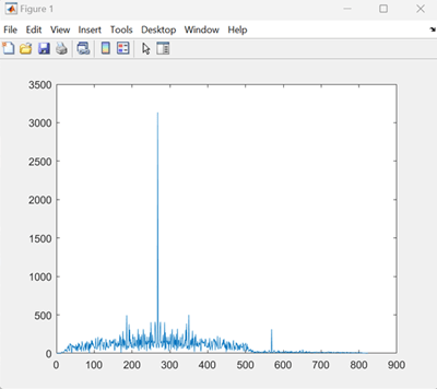
figure(1)
plot(abs(corrResult))

The peak in the graph corresponding to 0.2*refSignal is small
compared to the peak corresponding to 2*refSignal. The difference is
in the scaling values: 0.2 and 2. You also need to calculate the correlation result
appropriately if there are no known scaling values.
To remove the effects of scaling factors 0.2 and
2, you can use the fact that for any column vectors u and v,
abs(u'*v)/sqrt((u'*u)*(v'*v)) is always between 0 and 1. In this scenario, u is
refSignal and v is a moving slice of waveform. Compute and store
the magnitude squared of the waveform using a sliding window. Normalize the correlation
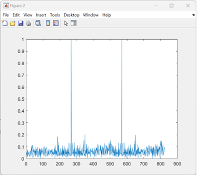
magnitude to get two peaks very close to
1.
% Calculate the magnitude squared of the waveform using a sliding window.
waveformMagSq = filter(ones(size(refSignal)),1,[real(waveform.*conj(waveform)); zeros(length(refSignal)-1, 1)]);

% Calculate the power of the reference signal.
refSigPower = real(refSignal'*refSignal);

% Normalize the correlation magnitude.
normCorrMag = abs(corrResult) ./ sqrt(waveformMagSq * refSigPower);

% Create a new figure for plotting
figure(2)

% Plot the normalized correlation magnitude.
plot(normCorrMag)

The timingEstimate function uses the above algorithm. The
function normalizes the correlation magnitude for each waveform from each receive
antenna (1:R) and each reference signal from each transmit layer (1:P).
If one such normalization vector has a value that is equal to or greater than the detection threshold, then the function decides that the reference signal is present in the received waveform. To understand more about detection threshold, see Estimate Timing Offset of QPSK Signals.
After confirming the presence of the reference signal in the received waveform, you need to estimate the timing offset You can use the autocorrelation properties of the reference signal to estimate the timing offset. Consider this example:
Generate a complex Gaussian noise reference signal with a specified scale factor. The scale factor of 3.4 is arbitrary and does not need to represent unit power.
refSignal = 3.4*randn(256,1,'like',1j);Calculate the total energy of the reference signal by taking the conjugate transpose of the signal.
refTotalEnergy = real(refSignal'*refSignal);
Simulate the effect of the channel on the reference signal by filtering it with a given channel impulse response. The filter coefficients [0.8 0.5+0.2j -0.3+0.4j] represent the channel.
waveform = filter([0.8 0.5+0.2j -0.3+0.4j], 1, refSignal);
Add complex Gaussian noise to the waveform to simulate a noisy channel. The noise has a standard deviation of 0.01, scaled by the waveform's size.
waveform = waveform + 0.01*randn(size(waveform), 'like', 1j);
Perform cross-correlation between the received waveform and the reference signal. For this, filter the received waveform with the time-reversed and conjugated reference signal. The result is equivalent to the cross-correlation function without padding zeros at the end.
corrResult = filter(conj(flipud(refSignal)), 1, [waveform;zeros(length(refSignal)-1, 1)]);
Estimate the channel impulse response by normalizing the cross-correlation result with the total energy of the reference signal.
estImpulseResponse = corrResult / refTotalEnergy;
Extract the estimated channel impulse response starting from the sample immediately after the reference signal length. This portion of the impulse response should be close to the actual channel filter coefficients. Add the length of the reference signal to the index to account for the delay introduced by the filtering process.
estImpulseResponse(length(refSignal)+(0:2))
The result is expected to be close to [0.8; 0.5+0.2j; -0.3+0.4j]
In the above example, the computation assumes that the reference signal has good autocorrelation properties or the autocorrelation function is close to an impulse, and that the reference signal is present in the received waveform.
The timingEstimate function calculates estimated impulse
response for each waveform from each receive antenna (1:R) and each reference signal
from each transmit layer (1:P), and then the function sums the magnitude squared of the
estimated impulse response over all R*P combinations.
The function uses this vector of total power to find which W consecutive samples in this vector have the largest sum. Here, W is the width of the window used to sum the power of estimated impulse response components. Subtracting the length of the reference signal from the one-based index of the first sample in these W consecutive samples gives the timing estimate. (If more than one set of W consecutive samples achieves the largest sum, then the smallest timing estimate is used.)
If W=1, the algorithm looks for a single peak in the total power vector.
If W>1, the algorithm considers a peak energy that spreads over multiple samples instead of one sample. You can set W to CPLEN+1, where CPLEN is the cyclic prefix length of an OFDM symbol. This region is the potential start of the OFDM symbol. This algorithm is a heuristic to reduce intersymbol interference.
This algorithm provides a practical means to estimate the timing offset in a communication system by leveraging the autocorrelation properties of a reference signal and the received waveform's cross-correlation with it.
Extended Capabilities
This function supports GPU array inputs. For more information, see Accelerate Simulation Using GPUs.
Version History
Introduced in R2024aThe timingEstimate function adds support for gpuArray (Parallel Computing Toolbox) object processing to run code on a graphics processing unit
(GPU).
MATLAB Command
You clicked a link that corresponds to this MATLAB command:
Run the command by entering it in the MATLAB Command Window. Web browsers do not support MATLAB commands.
Seleziona un sito web
Seleziona un sito web per visualizzare contenuto tradotto dove disponibile e vedere eventi e offerte locali. In base alla tua area geografica, ti consigliamo di selezionare: .
Puoi anche selezionare un sito web dal seguente elenco:
Come ottenere le migliori prestazioni del sito
Per ottenere le migliori prestazioni del sito, seleziona il sito cinese (in cinese o in inglese). I siti MathWorks per gli altri paesi non sono ottimizzati per essere visitati dalla tua area geografica.
Americhe
- América Latina (Español)
- Canada (English)
- United States (English)
Europa
- Belgium (English)
- Denmark (English)
- Deutschland (Deutsch)
- España (Español)
- Finland (English)
- France (Français)
- Ireland (English)
- Italia (Italiano)
- Luxembourg (English)
- Netherlands (English)
- Norway (English)
- Österreich (Deutsch)
- Portugal (English)
- Sweden (English)
- Switzerland
- United Kingdom (English)