Sources

Data Sources

To generate random data that simulates a signal source in your communications system, use the applicable functions and blocks listed in Communications Toolbox™.

Random Integers

In MATLAB®, the randi function generates random integer matrices whose entries are in a range that you specify. A special case generates random binary matrices.

For example, the command below generates a 5-by-4 matrix containing random integers between 2 and 10.

c = randi([2,10],5,4)

c = 5×4

     9     2     3     3
    10     4    10     5
     3     6    10    10
    10    10     6     9
     7    10     9    10

If your desired range is [0,10] instead of [2,10], you can use these commands to produce different numerical results that use the same distribution.

d = randi([0,10],5,4);
e = randi([0 10],5,4);

In Simulink®, the Random Integer Generator and Poisson Integer Generator blocks both generate vectors containing random nonnegative integers. The Random Integer Generator block uses a uniform distribution on a bounded range that you specify in the block mask. The Poisson Integer Generator block uses a Poisson distribution to determine its output. In particular, the output can include any nonnegative integer.

Random Symbols

The randsrc function generates random matrices whose entries are chosen independently from an alphabet that you specify, with a distribution that you specify. A special case generates bipolar matrices.

For example, the command below generates a 5-by-4 matrix whose entries are random, independently chosen, and uniformly distributed in the set {1,3,5}.

a = randsrc(5,4,[1,3,5])

a = 5×4

     5     5     5     3
     1     3     1     1
     3     1     5     1
     5     1     1     3
     5     1     5     3

To skew the distribution so that 1 is twice as likely to occur as either 3 or 5, use the following command. The third input argument has two rows, one of which indicates the possible values of b and the other indicates the probability of each value.

b = randsrc(5,4,[1,3,5; .5,.25,.25])

b = 5×4

     1     1     1     1
     5     5     1     3
     3     5     3     1
     3     1     5     1
     5     3     5     1

Random Bit Error Patterns

In MATLAB, the randerr function generates matrices whose entries are either 0 or 1. However, its options are different from those of randi because randerr is meant for testing error-control coding. For example, the command below generates a 5-by-4 binary matrix, where each row contains exactly one 1.

f = randerr(5,4)

f = 5×4

     0     0     0     1
     1     0     0     0
     1     0     0     0
     0     0     1     0
     0     0     0     1

You might use such a command to perturb a binary code that consists of five 4-bit codewords. Adding the random matrix f to your code matrix (modulo 2) introduces exactly one error into each codeword.

On the other hand, to perturb each codeword by introducing one error with probability 0.4 and two errors with probability 0.6, use the following command instead.

g = randerr(5,4,[1,2; 0.4,0.6])

g = 5×4

     1     0     1     0
     0     1     0     1
     0     0     0     1
     1     0     0     1
     0     0     1     0

Adding the random matrix g to your code matrix (modulo 2) introduces one or two errors into each codeword with the specified probability of occurrence for each. The probability matrix that is the third argument of randerr affects only the number of 1s in each row, not their placement.

As another application, you can generate an equiprobable binary 100-element column vector using any of the following commands. The three commands produce different numerical outputs that have the same distribution. The arguments vary according to the way each function specifies its behavior.

binarymatrix1 = randsrc(100,1,[0 1]); % Possible values are 0,1
binarymatrix2 = randi([0 1],100,1); % Two possible values
binarymatrix3 = randerr(100,1,[0 1; 0.5 0.5]); % No 1s, or one 1

In Simulink, the Bernoulli Binary Generator block generates random bits and is suitable for representing sources. The block considers each element of the signal to be an independent Bernoulli random variable. Also, different elements do not need to be identically distributed.

Sequence Generators

To generate sequences for spreading or synchronization in your communications system, use the applicable functions and blocks listed in Communications Toolbox™. You can generate pseudorandom sequences, synchronization codes, and orthogonal codes. For examples that compare the correlation properties of these sequence generators, see Spreading Sequences.

Pseudorandom Sequences

You can generate pseudorandom or pseudonoise (PN) sequences by using a System object™ in MATLAB^® or a block in Simulink^®. Communications system applications using these sequences include multiple-access spread spectrum, ranging, synchronization, and data scrambling. This table lists the types of pseudorandom sequences that you can use and the features that implement them:

Sequence	System Object	Block
Gold sequences	comm.GoldSequence	Gold Sequence Generator
Kasami sequences	comm.KasamiSequence	Kasami Sequence Generator
PN sequences	comm.PNSequence	PN Sequence Generator

To generate pseudorandom sequences, the underlying code implements shift registers, as illustrated in this diagram.

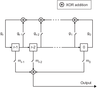
All r registers in the generator update their values at each time step according to the value of the incoming arrow to the shift register. The adders perform addition modulo 2. The shift register can be described by a binary polynomial in z, g_rz^r + g_r-1z^r-1 + ... + g₀. Between the ith shift register and the adder, the coefficient g_i is 1 if there is a connection, or 0 if there is no connection.

Between the ith shift register and the adder preceding the output, the coefficient m_i is 1 if there is a delay, or a 0 if there is no delay. If the shift is zero, the m₀ switch is closed while all other m_k switches are open.

The Kasami and PN sequence generators use this polynomial description for their generator polynomial. The Gold sequence generator uses this polynomial description for the preferred first and second generator polynomial PN sequences.

Model PN Sequence Generation with Linear Feedback Shift Register

Sequences output from the PN Sequence Generator block can be modeled using a linear feedback shift register (LFSR) built with primitive Simulink® blocks.

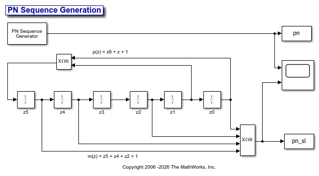
The cm_ex__pnseq_vs_prim_sl model generates the generator polynomial, p(z)=z^6+z+1, by using the PN Sequence Generator block and by modeling an LFSR using primitive Simulink blocks. The discrete block LFSR schematic model interprets the Initial states and Output mask vector (or scalar shift value) parameters of the PN Sequence Generator block. The PreLoadFcn callback function initializes runtime parameters. To view the callback functions from the Simulink Toolstrip, on the Modeling tab, in the Design gallery, click Property Inspector.

The scope output shows that the two implementations produce matching PN sequences.

Using the PN Sequence Generator block allows you to easily generate PN sequences of large periods. To experiment further, open the model. Modify settings to see how the performance varies for different path delays or adjust the PN sequence generator parameters. You can experiment with different initial states by changing the value of Initial states before running the simulation. For all values, the two generated sequences are the same.

Synchronization Codes

Use the comm.BarkerCode System object and Barker Code Generator block to generate Barker codes to perform synchronization. Characteristics that define Barker codes include:

• The code must be a subset of a PN sequence.

• The code must be a short code, with a maximum length of 13.

• The code must have low-correlation sidelobes. A correlation sidelobe is the correlation of a codeword with a time-shifted version of itself.

Orthogonal Codes

Orthogonal codes have perfect correlation properties, which makes them beneficial for use in spreading codes. In multi-user spread spectrum systems, where the receiver is perfectly synchronized with the transmitter, orthogonal codes are ideal for despreading operations. This table lists orthogonal codes and the features that you can use to implement them:

Code	System Object	Block
Hadamard codes	comm.HadamardCode	Hadamard Code Generator
OVSF codes	comm.OVSFCode	OVSF Code Generator
Walsh codes	comm.WalshCode	Walsh Code Generator

Noise Sources

Construct different types of channel noise in communication links by using these features:

Distribution	Function	Block
Gaussian	wgn	MATLAB Function (Simulink) block
Rayleigh	randn
Rician	randn
Uniform on a bounded interval	rand

Gaussian Noise Generator

In MATLAB®, the wgn function generates random matrices using a white Gaussian noise distribution. You specify the power of the noise in either dBW (decibels relative to a watt), dBm, or linear units. You can generate either real or complex noise.

For example, the command below generates a column vector of length 50 containing real white Gaussian noise whose power is 2 dBW. By default, the power type in dBW and load impedance is 1 ohm.

y1 = wgn(50,1,2);

To generate complex white Gaussian noise whose power is 2 watts, across a load of 60 ohms, use either of the commands below.

y2 = wgn(50,1,2,60,'complex','linear');
y3 = wgn(50,1,2,60,'linear','complex');

To send a signal through an additive white Gaussian noise channel, use the awgn function. See AWGN Channel for more information.

Random Noise Generators

In Simulink®, you can construct random noise generators to simulate channel noise by using the MATLAB® Function block with the desired random number generator function. This example generates and displays histogram plots of Gaussian, Rayleigh, Rician, and uniform noise.

The cm_ex_random_noise_generation model contains noise generators configured to output -by-1 vectors every second, which is equivalent to a 0.00001 second sample time. In this model, each MATLAB Function block defines a specific noise generator using its underlying function. You can view the underlying code for a MATLAB Function block by selecting the desired MATLAB Function block in the model, and then press Ctrl+u. Each MATLAB Function block contains block mask parameters that map to the function arguments in the underlying code.

For each MATLAB Function block, the Samples per frame parameter maps to its underlying function argument, spf. Similarly, Seed maps to seed.

The Gaussian Noise MATLAB Function block maps the Power (dBW) parameter to p, and defines this function:

The Rayleigh Noise MATLAB Function block maps the Sigma parameter to alpha, and defines this function:

The Rician Noise MATLAB Function block maps the Rician K-factor parameter to K and the Sigma parameter to s, and defines this function:

The Uniform Noise MATLAB Function block maps the Noise lower bound parameter to lb and the Noise upper bound parameter to ub, and defines this function:

The model generates these histogram plots to show the noise distribution across the spectrum for each noise generator.

To explore further, open the model and adjust one of the noise generation settings. For example, the Rician noise generator has a K-factor of 10, which causes the mean value of the noise to be larger than that of the Rayleigh distributed noise. Double-click the Rician Noise MATLAB Function block to open the block mask and change the K-factor from 10 to 2. Rerun the model to see the noise spectrum shift.