spectralfact

Spectral factorization of linear systems

Syntax

[G,S] = spectralfact(H)

[G,S] = spectralfact(F,R)

G = spectralfact(F,[])

Description

[G,S] = spectralfact(H) computes the spectral factorization:

H = G'*S*G

of an LTI model satisfying H = H'. In this factorization, S is a symmetric matrix and G is a square, stable, and minimum-phase system with unit (identity) feedthrough. G' is the conjugate of G, which has transfer function G(–s)^T in continuous time, and G(1/z)^T in discrete time.

[G,S] = spectralfact(F,R) computes the spectral factorization:

F'*R*F = G'*S*G

without explicitly forming H = F'*R*F. As in the previous syntax, S is a symmetric matrix and G is a square, stable, and minimum-phase system with unit feedthrough.

G = spectralfact(F,[]) computes a stable, minimum-phase system G such that:

G'*G = F'*F.

Examples

Spectral Factorization of System

Consider the following system.

G0 = ss(zpk([-1 -5 1+2i 1-2i],[-100 1+2i 1-2i -10],1e3));
H = G0'*G0;

G0 has a mix of stable and unstable dynamics. H is a self-conjugate system whose dynamics consist of the poles and zeros of G0 and their reflections across the imaginary axis. Use spectral factorization to separate the stable poles and zeros into G and the unstable poles and zeros into G'.

[G,S] = spectralfact(H);

Confirm that G is stable and minimum phase, by checking that all its poles and zeros fall in the left half-plane (Re(s) < 0).

p = pole(G)

p = 4×1 complex
102 ×

  -0.0100 + 0.0200i
  -0.0100 - 0.0200i
  -0.1000 + 0.0000i
  -1.0000 + 0.0000i

z = zero(G)

z = 4×1 complex

  -1.0000 + 2.0000i
  -1.0000 - 2.0000i
  -1.0000 + 0.0000i
  -5.0000 + 0.0000i

G also has unit feedthrough.

G.D

ans = 
1

Because H is SISO, S is a scalar. If H were MIMO, the dimensions of S would match the I/O dimensions of H.

S

S = 
1000000

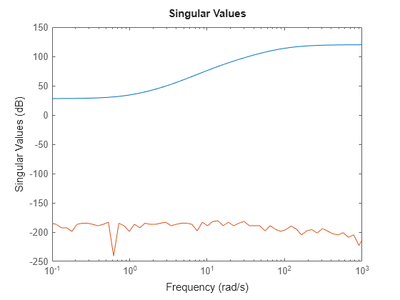
Confirm that G and S satisfy H = G'*S*G by comparing the original system to the difference between the original and factored systems. sigmaplot throws a warning because the difference is very small.

Hf = G'*S*G;
sigmaplot(H,H-Hf)

Warning: The frequency response has poor relative accuracy. This may be because the response is nearly zero or infinite at all frequencies, or because the state-space realization is ill conditioned. Use the "prescale" command to investigate further.

Spectral Factorization from Factored Form

Suppose that you have the following 2-output, 2-input state-space model, F.

A = [-1.1  0.37;
     0.37 -0.95];
B = [0.72 0.71;
     0    -0.20];
C =  [0.12 1.40
      1.49 1.41];
D = [0.67 0.7172;
    -1.2  0];
F = ss(A,B,C,D);

Suppose further that you have a symmetric 2-by-2 matrix, R.

R =   [0.65    0.61
       0.61   -3.42];

Compute the spectral factorization of the system given by H = F'*R*F, without explicitly computing H.

[G,S] = spectralfact(F,R);

G is a minimum-phase system with identity feedthrough.

G.D

ans = 2×2

     1     0
     0     1

Because F is has two inputs and two outputs, both R and S are 2-by-2 matrices.

Confirm that G'*S*G = F'*R*F by comparing the original factorization to the difference between the two factorizations. The singular values of the difference are far below those of the original system.

Ff = F'*R*F;
Gf = G'*S*G;
sigmaplot(Ff,Ff-Gf)

Implicit Factorization

Consider the following discrete-time system.

F = zpk(-1.76,[-1+i -1-i],-4,0.002);

F has poles and zeros outside the unit circle. Use spectralfact to compute a system G with stable poles and zeros, such that G'*G = F'*F.

G = spectralfact(F,[])

G =
 
  -3.52 z (z+0.5682)
  ------------------
   (z^2 + z + 0.5)
 
Sample time: 0.002 seconds
Discrete-time zero/pole/gain model.

Unlike F, G has no poles or zeroes outside the unit circle. G does have an additional zero at z = 0, which is a reflection of the unstable zero at z = Inf in F.

pzplot(G)

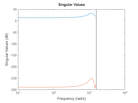
Confirm that G'*G = F'*F by comparing the original factorization to the difference between the two factorizations. The singular values of the difference are far below those of the original factorization.

Ff = F'*F;
Gf = G'*G;
sigmaplot(Ff,Ff-Gf)

Input Arguments

H — Self-conjugate LTI model

tf | zpk | ss

Self-conjugate LTI model, specified as a tf, ss, or zpk model. Self-conjugate means that is equal to its conjugate, H = H'. The conjugate H' is the transfer function H(–s)^T in continuous time and H(1/z)^T in discrete time.

H can be SISO or MIMO, provided it has as many outputs as inputs. H can be continuous or discrete with the following restrictions:

• In continuous time, H must be biproper with no poles or zeros at infinity or on the imaginary axis.

• In discrete time, H must have no poles or zeros on the unit circle.

F — F factor

tf | zpk | ss

F factor of the factored form H = F'*R*F, specified as a tf, ss, or zpk model. F cannot have more inputs than outputs.

R — R factor

square matrix

R factor of the factored form H = F'*R*F, specified as a symmetric square matrix with as many rows as there are outputs in F.

Output Arguments

G — LTI factor

tf | zpk | ss

LTI factor, returned as a tf, ss, or zpk model. G is a stable, minimum-phase system that satisfies:

• H = G'*S*G, if you use the syntax [G,S] = spectralfact(H).

• G'*S*G = F'*R*F, if you use the syntax [G,S] = spectralfact(F,R).

• G'*G = F'*F, if you use the syntax G = spectralfact(F,[]).

S — Numeric factor

matrix

Numeric factor, returned as a symmetric matrix that satisfies:

• H = G'*S*G, if you use the syntax [G,S] = spectralfact(H). The dimensions of S match the I/O dimensions of H and G.

• G'*S*G = F'*R*F, if you use the syntax [G,S] = spectralfact(F,R). The size of S along each dimension matches the number of outputs of F.

Tips

• spectralfact assumes that H is self-conjugate. In some cases when H is not self-conjugate, spectralfact returns G and S that do not satisfy H = G'*S*G. Therefore, verify that your input model is in fact self-conjugate before using spectralfact. One way to verify H is to compare H to H - H' on a singular value plot.

  sigmaplot(H,H-H')

  If H is self-conjugate, the H - H' line on the plot lies far below the H line.

Version History

Introduced in R2016a