Main Content

view

Plot mode information when using modal truncation method

Since R2023b

    Description

    Use view to graphically analyze the model and select a model order reduction criteria from a model order reduction task created using reducespec. For ModalTruncation and SparseModalTruncation objects, you can visualize modes (poles) based on their locations, damping and natural frequencies, or normalized DC contributions. For the full workflow, see Task-Based Model Order Reduction Workflow.

    view(R,type) creates a plot that helps you select the modal content of the reduced model. R specifies the model order reduction (MOR) specification object. Use the type argument to specify these plot types.

    • "mode" — Mode locations

    • "damp" — Mode damping and natural frequencies

    • "contrib" — Bar chart of normalized DC contributions

    example

    view(R) plots the default plot type for the model order reduction algorithm of R. For the modal truncation method, this syntax plots the mode locations.

    view(___,Axes=AX) plots on the Axes object in the current figure with the handle AX. Use this input argument after any of the input argument combinations in the previous syntaxes. For more information about customizing axes, see Axes Properties.

    example

    h = view(___) returns a plot handle h. Use h to modify properties of the plot after creating it.

    example

    view(R,"-help") returns help specific to the model order specification object R. The returned help shows plot types and syntaxes applicable to R.

    Examples

    collapse all

    This example shows how to obtain a reduced-order model of a structural beam using the modal truncation method. For this example, consider a SISO sparse state-space model of a cantilever beam. This example uses the linearized model from the Linear Analysis of Cantilever Beam example.

    Load the beam model.

    load linBeam.mat
    size(sys)
    Sparse second-order model with 1 outputs, 1 inputs, and 3303 degrees of freedom.
    

    Plot the Bode response.

    bode(sys,w)

    MATLAB figure

    Create a model order reduction task.

    R = reducespec(sys,"modal");

    Set the Focus option to compute the eigenvalues only in the specified frequency range.

    R.Options.Focus = [0 5e5];

    Analyze the model and compute the derived information.

    R = process(R);
    size(R.Mode)
    ans = 1×2
    
        26     1


    The original model contains 26 modes. View the DC contribution of the modal components using the view function.

    view(R,"contrib")

    Figure contains an axes object. The axes object with title DC Contribution of Modal Components, xlabel Modal Component (Sorted), ylabel Normalized DC Contribution contains an object of type bar.

    Discard the modes with smaller contributions. For this example, discard all modes with DC contribution smaller than 1e-6. This results in a reduced model with 12 modes.

    [rsys,info] = getrom(R,MinDC=1e-6);

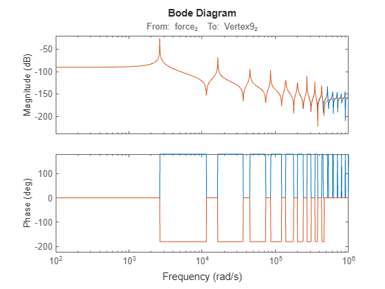
    Plot the bode responses.

    bode(sys,rsys,w)

    MATLAB figure

    The reduced-order model provides a good approximation for the original sparse model.

    This example shows how customize the plots of modal components obtained using the view function.

    For this example, create a model order reduction specification for an LTI model using the modal truncation method. Generate a random discrete-time state-space model with 40 states.

    rng(0)
    sys = drss(40);

    Create a specification object.

    R = reducespec(sys,"modal");

    Visualize the DC contributions of the modes.

    view(R,"contrib")

    Figure contains an axes object. The axes object with title DC Contribution of Modal Components, xlabel Modal Component (Sorted), ylabel Normalized DC Contribution contains an object of type bar.

    To customize the plots for the modal truncation method, you can use an Axes object.

    figure
    ax1 = axes('Position',[0.1 0.1 0.7 0.7]);
    ax2 = axes('Position',[0.65 0.45 0.28 0.28]);
    h1 = view(R,"contrib",Axes=ax1);
    h2 = view(R,"damp",Axes=ax2);

    To further customize the plots, use the plot handles to set the options.

    h2.YScale = "linear";
    h1.FontWeight = "bold";

    Figure contains 2 axes objects. Axes object 1 with title DC Contribution of Modal Components, xlabel Modal Component (Sorted), ylabel Normalized DC Contribution contains an object of type bar. Axes object 2 with title Mode Damping and Natural Frequency, xlabel Damping, ylabel Natural Frequency contains a line object which displays its values using only markers.

    Input Arguments

    collapse all

    Model order reduction specification object created using reducespec, specified as a ModalTruncation or SparseModalTruncation object.

    Plot type, specified as one of the following.

    • "mode" — Mode locations

    • "damp" — Mode damping and natural frequencies

    • "contrib" — Bar chart of normalized DC contributions

    If you do not specify this argument, the function plots the mode locations of the original system sys.

    Output Arguments

    collapse all

    Plot handle object, returned as an Axes object.

    Use dot notation with this handle to customize the plot. For example, h.YScale = "Linear". For a list of available options, see Axes Properties.

    Version History

    Introduced in R2023b

    Go to top of page