viewGoal
View tuning goals; validate design against tuning goals
Description
viewGoal( displays a graphical view of a tuning
goal or vector of tuning goals, specified as Req)TuningGoal objects.
The form of the tuning-goal plot depends on the specific tuning goals you use. Plots
for time-domain tuning goals typically show the target time-domain response
specified in the tuning goal. Plots for frequency-domain tuning goals typically show
a shaded area that represents the region in which the tuning goal is
violated.
When you provide a vector of tuning goals, viewGoal plots each
tuning goal on separate axes in a single figure window.
viewGoal( plots the
performance of a tuned control system against the tuning goal or goals. The form of
the tuning-goal plot depends on the specific tuning goals you use. Typically, the
plot shows both the target response specified in the tuning goal and the
corresponding response of the control system represented by Req,T)T.
For more information about interpreting tuning-goal plots, see Visualize Tuning Goals.
Examples
Create a tuning goal that constrains the response from a signal 'd' to another signal 'y' to roll off at 20 dB/decade at frequencies greater than 1. The tuning goal also imposes disturbance rejection (maximum gain of 1) in the frequency range [0,1].
gmax = frd([1 1 0.01],[0 1 100]);
Req = TuningGoal.MaxGain('du','u',gmax);
When you use a frequency response data (frd) model to sketch the bounds of a gain constraint or loop shape, the tuning goal interpolates the constraint. This interpolation converts the constraint to a smooth function of frequency. Examine the interpolated gain constraint using viewGoal.
viewGoal(Req)
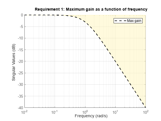
The dotted line shows the gain profile specified in the tuning goal. The shaded region represents gain values that violate the tuning requirement. For more information about interpreting tuning-goal plots, see Visualize Tuning Goals.
Examine the tuned response of a control system against tuning goals, to determine where and by how much the tuning goals are violated. This visualization helps you determine whether the tuned control system comes satisfactorily close to meeting your soft requirements.
Open a Simulink® model of a control system to tune.
open_system('rct_airframe2')
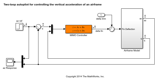
Create tuning goals. For this example, use tracking, roll-off, stability margin, and disturbance-rejection tuning goals.
Req1 = TuningGoal.Tracking('az ref','az',1);
Req2 = TuningGoal.Gain('delta fin','delta fin',tf(25,[1 0]));
Req3 = TuningGoal.Margins('delta fin',7,45);
MaxGain = frd([2 200 200],[0.02 2 200]);
Req4 = TuningGoal.Gain('delta fin','az',MaxGain);
Create an slTuner interface, and tune the model with these tuning goals designated as soft goals.
ST0 = slTuner('rct_airframe2','MIMO Controller');
addPoint(ST0,'delta fin');

rng('default');
[ST1,fSoft] = systune(ST0,[Req1,Req2,Req3,Req4]);
Final: Soft = 1.13, Hard = -Inf, Iterations = 97
Verify that the tuned system satisfies the margin requirement.
figure;
viewGoal(Req3,ST1)
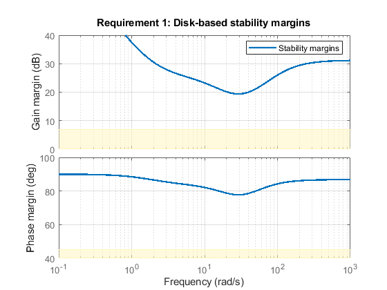
The shaded region corresponds to margins falling short of the target of 7 dB gain margin and 45 degrees phase margin. The solid line shows that the margin requirement is satisfied at all frequencies.
Examine system responses compared to the tracking and disturbance-rejection tuning goals. When you provide a vector of tuning goals, viewGoal plots them on separate axes in a single figure.
figure
viewGoal([Req1,Req4],ST1)
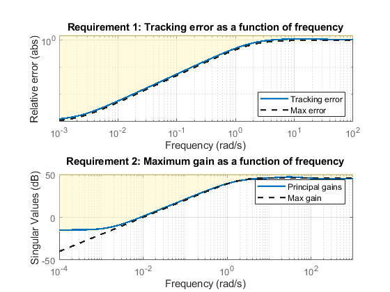
The first plot shows that the tuned system response very nearly satisfies the tracking requirement. The slight violation suggests that setpoint tracking will perform close to expectations.
The second plot shows that the gain requirement is satisfied except at low frequency. For this tuning goal, the shaded region, which represents the effective tuning constraint, diverges from the specified maximum gain profile at low frequency. This modification to the gain profile is to avoid a pole at s = 0 in the weighting function used to normalize the goal (see Tips on this page). While the tuned gain exceeds the specified gain below 0.001 rad/s, it is still about 60 dB less than the peak value, which is typically enough in practice.
To further examine the responses of the tuned system, use getIOTransfer to extract the relevant transfer functions for analysis with time-domain commands such as step.
Input Arguments
Tips
For general information about how to interpret tuning-goal plots, see Visualize Tuning Goals. For information about interpreting margin-goal plots in particular, see Stability Margins in Control System Tuning.
For varying tuning goals that you create with
varyingGoal, the tuning-goal plot generated byviewGoallets you examine the tuning goal at each design point. For more information, see Validate Gain-Scheduled Control Systems.With some frequency-domain tuning goals, there might be a difference between the gain profile you specify in the tuning goal (dashed line), and the profile the software uses for tuning (shaded region). In this case, the shaded region of the plot reflects the profile that the software uses for tuning. The gain profile you specify and the gain profile used for tuning might differ if:
You tune a control system in discrete time, but specify the gain profile in continuous time.
The software modifies the asymptotes of the specified gain profile to improve numeric stability.
For more information about how an enforced tuning goal might differ from the goal, see Visualize Tuning Goals.
For MIMO feedback loops, the
LoopShape,MinLoopGain,MaxLoopGain,Margins,Sensitivity, andRejectiongoals are sensitive to the relative scaling of each SISO loop.systunetries to balance the overall loop-transfer matrix while enforcing such goals. The optimal loop scaling is stored in the tuned closed-loop model orslTunerinterfaceTreturned bysystune. For consistency,viewGoal(R,T)takes this scaling into account, and plots the scaled open-loop response or sensitivity. To omit this scaling, useviewGoal(R,clearTuningInfo(T)).Modifying
Tmight compromise the validity of the stored scaling. Therefore, if you make significant modifications toT, retuning is recommended to update the scaling data.
Version History
Introduced in R2017b
See Also
systune | genss | evalGoal | systune (for slTuner) (Simulink Control Design)