Mark Analysis Points in Closed-Loop Models
This example shows how to build a block diagram and insert analysis points at locations of interest using the connect command. You can then use the analysis points to extract various system responses from the model.
For this example, create a model of a Smith predictor, the SISO multiloop control system shown in the following block diagram.
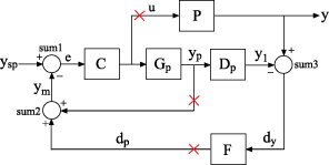
Points marked by x are analysis points to mark for this example. For instance, if you want to calculate the step response of the closed-loop system to a disturbance at the plant input, you can use an analysis point at u. If you want to calculate the response of the system with one or both of the control loops open, you can use the analysis points at yp or dp.
To build this system, first create the dynamic components of the block diagram. Specify names for the input and output channels of each model so that connect can automatically join them to build the block diagram.
s = tf('s');

% Process model
P = exp(-93.9*s) * 5.6/(40.2*s+1);
P.InputName = 'u';
P.OutputName = 'y';

% Predictor model
Gp = 5.6/(40.2*s+1);
Gp.InputName = 'u';
Gp.OutputName = 'yp';

% Delay model
Dp = exp(-93.9*s);
Dp.InputName = 'yp';
Dp.OutputName = 'y1';

% Filter
F = 1/(20*s+1);
F.InputName = 'dy';
F.OutputName = 'dp';

% PI controller
C = pidstd(0.574,40.1);
C.Inputname = 'e';
C.OutputName = 'u';
Create the summing junctions needed to complete the block diagram. (For more information about creating summing junctions, see sumblk).
sum1 = sumblk('e = ysp - ym');
sum2 = sumblk('ym = yp + dp');
sum3 = sumblk('dy = y - y1');
Assemble the complete model.
input = 'ysp';
output = 'y';
APs = {'u','dp','yp'};
T = connect(P,Gp,Dp,C,F,sum1,sum2,sum3,input,output,APs)
Generalized continuous-time state-space model with 1 outputs, 1 inputs, 4 states, and the following blocks:
  CONNECT_AP1: Analysis point, 3 channels, 1 occurrences.
Model Properties

Type "ss(T)" to see the current value and "T.Blocks" to interact with the blocks.
When you use the APs input argument, the connect command automatically inserts an AnalysisPoint block into the generalized state-space (genss) model, T. The automatically generated block is named AnalysisPoints_. The three channels of AnalysisPoints_ correspond to the three locations specified in the APs argument to the connect command. Use getPoints to see a list of the available analysis points in the model.
getPoints(T)
ans = 3×1 cell
    {'dp'}
    {'u' }
    {'yp'}
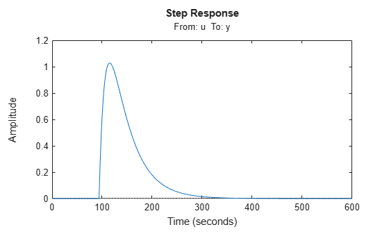
Use these locations as inputs, outputs, or loop openings when you extract responses from the model. For example, extract and plot the response at the system output to a step disturbance at the plant input, u.
Tp = getIOTransfer(T,'u','y');
stepplot(Tp)
Similarly, calculate the open-loop response of the plant and controller by opening both feedback loops.
openings = {'dp','yp'};
L = getIOTransfer(T,'ysp','y',openings);
bodeplot(L)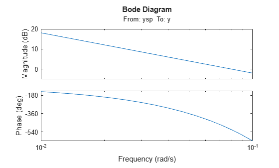
When you create a control system model, you can create an AnalysisPoint block explicitly and assign input and output names to it. You can then include it in the input arguments to connect as one of the blocks to combine. However, using the APs argument to connect as illustrated in this example is a simpler way to mark points of interest when building control system models.
See Also
connect | AnalysisPoint | sumblk