Designing Filters with Non-Equiripple Stopband
This example shows how to design lowpass filters with stopbands that are not equiripple.
Optimal Non-Equiripple Lowpass Filters
To start, set up the filter parameters and use fdesign to create a constructor for designing the filter.
N = 100;
Fp = 0.38;
Fst = 0.42;
Hf = fdesign.lowpass('N,Fp,Fst',N,Fp,Fst);
Equiripple designs achieve optimality by distributing the deviation from the ideal response uniformly. This has the advantage of minimizing the maximum deviation (ripple). However, the overall deviation, measured in terms of its energy tends to be large. This may not always be desirable. When low pass filtering a signal, this implies that remnant energy of the signal in the stopband may be relatively large. When this is a concern, least-squares methods provide optimal designs that minimize the energy in the stopband.
Hd1 = design(Hf,'equiripple',SystemObject=true);
Hd2 = design(Hf,'firls',SystemObject=true);
filterAnalyzer(Hd1,Hd2,FilterNames=["Equiripple design","Least-squares design"]);
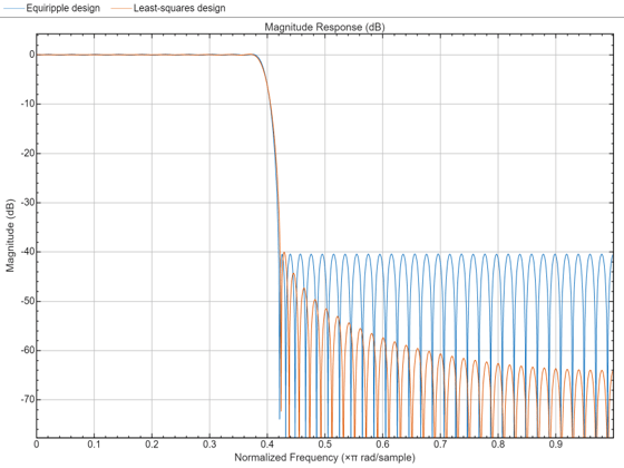
Notice how the attenuation in the stopband increases with frequency for the least-squares designs while it remains constant for the equiripple design. The increased attenuation in the least-squares case minimizes the energy in that band of the signal to be filtered.
Equiripple Designs with Increasing Stopband Attenuation
An often undesirable effect of least-squares designs is that the ripple in the passband region close to the passband edge tends to be large. For low pass filters in general, it is desirable that passband frequencies of a signal to be filtered are affected as little as possible. To this extent, an equiripple passband is generally preferable. If it is still desirable to have an increasing attenuation in the stopband, we can use design options for equiripple designs to achieve this.
Hd3 = design(Hf,'equiripple',StopbandShape='1/f',...
    StopbandDecay=4,SystemObject=true);
filterAnalyzer(Hd2,Hd3,FilterNames=["Least-Squares Design",...
    "Equiripple Design with Stopband Decaying as (1/f)^4"]);
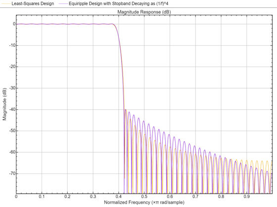
Notice that the stopbands are quite similar. However the equiripple design has a significantly smaller passband ripple,
mls = measure(Hd2);
meq = measure(Hd3);
mls.Apass
ans = 0.3504
meq.Apass
ans = 0.1867
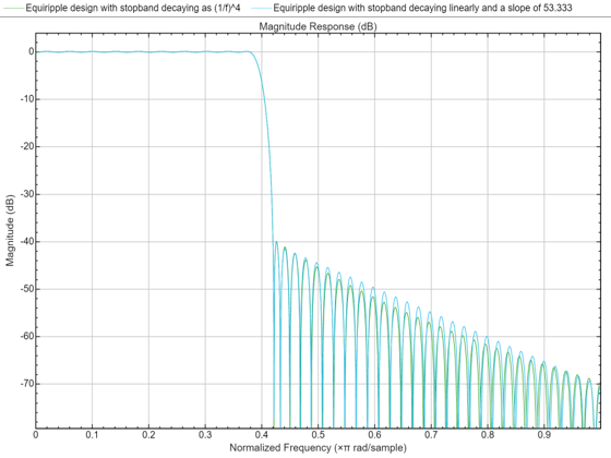
Filters with a stopband that decays as (1/f)^M will decay at 6M dB per octave. Another way of shaping the stopband is using a linear decay. For example given an approximate attenuation of 38 dB at 0.4*pi, if an attenuation of 70 dB is desired at pi, and a linear decay is to be used, the slope of the line is given by (70-38)/(1-0.4) = 53.333. Such a design can be achieved from:
Hd4 = design(Hf,'equiripple',StopbandShape='linear',...
    StopbandDecay=53.333,SystemObject=true);
filterAnalyzer(Hd3,Hd4,FilterNames=["Equiripple design with stopband decaying as (1/f)^4",...
    "Equiripple design with stopband decaying linearly and a slope of 53.333"]);
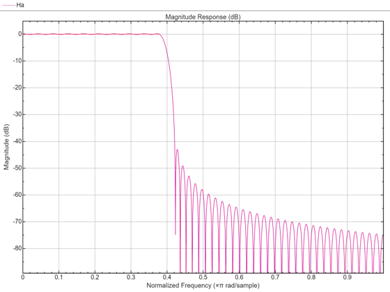
Yet another possibility is to use an arbitrary magnitude specification and select two bands (one for the passband and one for the stopband). Then, by using weights for the second band, it is possible to increase the attenuation throughout the band.
N = 100;
B = 2;  % number of bands
F = [0 .38 .42:.02:1];
A = [1 1 zeros(1,length(F)-2)];
W = linspace(1,100,length(F)-2);
Harb = fdesign.arbmag('N,B,F,A',N,B,F(1:2),A(1:2),F(3:end),...
    A(3:end));
Ha = design(Harb,'equiripple',B2Weights=W,...
    SystemObject=true);
filterAnalyzer(Ha)
You can also select a web site from the following list:
Americas
- América Latina (Español)
- Canada (English)
- United States (English)
Europe
- Belgium (English)
- Denmark (English)
- Deutschland (Deutsch)
- España (Español)
- Finland (English)
- France (Français)
- Ireland (English)
- Italia (Italiano)
- Luxembourg (English)
- Netherlands (English)
- Norway (English)
- Österreich (Deutsch)
- Portugal (English)
- Sweden (English)
- Switzerland
- United Kingdom (English)