Perform Data Type Optimization with Custom Behavioral Constraints

This example uses:

This example shows how to optimize fixed-point data types with fxpopt using custom behavioral constraints in the frequency domain. The Simulink® models in this example demonstrate two ways of using blocks from the Model Verification library to author custom behavioral constraints on the SNR (signal-to-noise ratio) of a low-pass filter. In the first example, calculate an approximation of the noise floor; in the second example, calculate the SNR difference between the original model and the quantized model that uses fixed-point data types.

Behavioral Constraints for Data Type Optimization

Data type optimization seeks to minimize an objective function, such as the total bit width, while maintaining original system behavior within a specified tolerance. During the optimization, the software establishes a baseline by simulating the original model. The software then constructs different fixed-point versions of your model and runs simulations to determine the behavior using the new data types. The optimization selects the model that minimizes the objective function while also meeting the specified behavioral constraints.

To determine if the behavior of a new fixed-point implementation is acceptable, the optimization requires well-defined behavioral constraints. You must specify at least one behavioral constraint. There are two ways to specify behavioral constraints for use with fxpopt:

1. Tolerance-based simulation comparisons to the baseline reference - You can add tolerances for signals that have signal logging enabled using the addTolerance method of fxpOptimizationOptions. A tolerance specifies an envelope of passing behavior with respect to the baseline simulation of the model.

2. Simulation-based assertion checks - You can use blocks in the Model Verification block library to author custom verification expressions. Enabled model verification blocks in your model are interpreted as behavioral constraints by the optimization solver.

You can also use a combination of signal tolerances and model verification blocks to specify behavioral constraints for your model. For more information, see Specify Behavioral Constraints.

Example 1: Calculate an Approximation of the Noise Floor

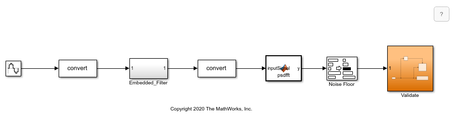
In this example, you convert a low-pass filter to use optimized fixed-point data types using fxpopt. To ensure that the embedded version still meets the SNR requirements, the model mLowPass_NoiseFloor contains additional logic to compute the noise floor of the signal at the output of the filter. This signal is then routed to the Validate subsystem, which uses a Check State Range block from the Model Verification block library. If the noise floor values calculated during simulation are outside the specified static range, fxpopt will interpret the model as not passing the behavioral constraints.

To begin, open the system for which you want to optimize the data types.

model = 'mLowPass_NoiseFloor';
sud = [model '/Embedded_Filter'];
open_system(model);

Use the fxpopt function to run the optimization. Because a model verification block is used to specify the constraints, it is not required to specify signal tolerances using the addTolerance method of fxpOptimizationOptions.

result = fxpopt(model,sud)

	+ Starting data type optimization...
	+ Checking for unsupported constructs.
	+ Preprocessing
	+ Modeling the optimization problem
		- Constructing decision variables
	+ Running the optimization solver
		- Evaluating new solution: cost 110, meets the behavioral constraints.
		- Updated best found solution, cost: 110
	+ Optimization has finished.
		- Neighborhood search complete.
		- Reached limit of number of iterations without updates to the current best solution.
	+ Fixed-point implementation that satisfies the behavioral constraints found. The best found solution is applied on the model.
		- Total cost: 110
		- Use the explore method of the result to explore the implementation.

result = 

  OptimizationResult with properties:

                  Model: 'mLowPass_NoiseFloor'
      SystemUnderDesign: 'mLowPass_NoiseFloor/Embedded_Filter'
           FinalOutcome: 'Fixed-point implementation that satisfies the behavioral constraints found. The best found solution is applied on the model.'
    OptimizationOptions: [1×1 fxpOptimizationOptions]
              Solutions: [1×1 DataTypeOptimization.OptimizationSolution]

Use the explore method to explore the design containing the optimized fixed-point data types.

explore(result);

Example 2: Calculate SNR Diffierence Between Original and Quantized Models

In this example, optimize fixed-point data types for the low-pass filter model, mLowPass_SNR, using a different set of behavioral constraints that compare the SNR of the embedded filter with the SNR of the original filter, which uses double-precision data types. The ValidateSNR subsystem first computes the SNR then uses a Check Static Lower Bound block from the Model Verification library to assert that the SNR is greater than 60. If the SNR drops below this specified value, then fxpopt will interpret the model as not passing the behavioral constraints.

To begin, open the system for which you want to optimize the data types.

model = 'mLowPass_SNR';
sud = [model '/Embedded_Filter'];
Source = 1;
open_system(model);

For this example, specify additional simulation scenarios by creating a Simulink.SimulationInput object. Use one sine wave input with a frequency of 100 rad/sec and a second sine wave input with a frequency of 500 rad/sec. fxpopt will consider both simulation scenarios during the optimization. A comprehensive set of input signals can help to ensure that the full operating range of your design is exercised during the optimization process.

si(1) = Simulink.SimulationInput(model);
si(1) = si(1).setVariable('Source',1);
si(2) = Simulink.SimulationInput(model);
si(2) = si(2).setVariable('Source',2);

Create an fxpOptimizationOptions object. Use the advanced options to define simulation scenarios to consider during optimization.

options = fxpOptimizationOptions();
options.AdvancedOptions.SimulationScenarios = si;

result = fxpopt(model,sud,options);

+ Starting data type optimization...
+ Checking for unsupported constructs.
+ Preprocessing
+ Modeling the optimization problem
- Constructing decision variables
+ Running the optimization solver
- Evaluating new solution: cost 112, does not meet the behavioral constraints.
- Evaluating new solution: cost 168, does not meet the behavioral constraints.
- Evaluating new solution: cost 224, does not meet the behavioral constraints.
- Evaluating new solution: cost 280, does not meet the behavioral constraints.
- Evaluating new solution: cost 336, does not meet the behavioral constraints.
- Evaluating new solution: cost 392, does not meet the behavioral constraints.
- Evaluating new solution: cost 448, does not meet the behavioral constraints.
- Evaluating new solution: cost 504, does not meet the behavioral constraints.
- Evaluating new solution: cost 560, does not meet the behavioral constraints.
- Evaluating new solution: cost 616, does not meet the behavioral constraints.
- Evaluating new solution: cost 672, does not meet the behavioral constraints.
- Evaluating new solution: cost 728, does not meet the behavioral constraints.
- Evaluating new solution: cost 784, does not meet the behavioral constraints.
- Evaluating new solution: cost 840, does not meet the behavioral constraints.
- Evaluating new solution: cost 896, does not meet the behavioral constraints.
- Evaluating new solution: cost 952, does not meet the behavioral constraints.
- Evaluating new solution: cost 1008, meets the behavioral constraints.
- Updated best found solution, cost: 1008
- Evaluating new solution: cost 995, meets the behavioral constraints.
- Updated best found solution, cost: 995
- Evaluating new solution: cost 994, meets the behavioral constraints.
- Updated best found solution, cost: 994
- Evaluating new solution: cost 993, meets the behavioral constraints.
- Updated best found solution, cost: 993
- Evaluating new solution: cost 992, meets the behavioral constraints.
- Updated best found solution, cost: 992
- Evaluating new solution: cost 991, meets the behavioral constraints.
- Updated best found solution, cost: 991
- Evaluating new solution: cost 990, meets the behavioral constraints.
- Updated best found solution, cost: 990
- Evaluating new solution: cost 989, meets the behavioral constraints.
- Updated best found solution, cost: 989
- Evaluating new solution: cost 988, meets the behavioral constraints.
- Updated best found solution, cost: 988
- Evaluating new solution: cost 987, meets the behavioral constraints.
- Updated best found solution, cost: 987
- Evaluating new solution: cost 986, meets the behavioral constraints.
- Updated best found solution, cost: 986
- Evaluating new solution: cost 985, meets the behavioral constraints.
- Updated best found solution, cost: 985
- Evaluating new solution: cost 984, meets the behavioral constraints.
- Updated best found solution, cost: 984
- Evaluating new solution: cost 982, meets the behavioral constraints.
- Updated best found solution, cost: 982
- Evaluating new solution: cost 981, does not meet the behavioral constraints.
- Evaluating new solution: cost 981, does not meet the behavioral constraints.
- Evaluating new solution: cost 981, does not meet the behavioral constraints.
- Evaluating new solution: cost 981, does not meet the behavioral constraints.
- Evaluating new solution: cost 981, does not meet the behavioral constraints.
- Evaluating new solution: cost 981, does not meet the behavioral constraints.
- Evaluating new solution: cost 981, meets the behavioral constraints.
- Updated best found solution, cost: 981
- Evaluating new solution: cost 980, meets the behavioral constraints.
- Updated best found solution, cost: 980
- Evaluating new solution: cost 979, does not meet the behavioral constraints.
- Evaluating new solution: cost 979, meets the behavioral constraints.
- Updated best found solution, cost: 979
- Evaluating new solution: cost 978, does not meet the behavioral constraints.
- Evaluating new solution: cost 978, meets the behavioral constraints.
- Updated best found solution, cost: 978
- Evaluating new solution: cost 977, does not meet the behavioral constraints.
- Evaluating new solution: cost 977, meets the behavioral constraints.
- Updated best found solution, cost: 977
- Evaluating new solution: cost 976, meets the behavioral constraints.
- Updated best found solution, cost: 976
- Evaluating new solution: cost 975, meets the behavioral constraints.
- Updated best found solution, cost: 975
- Evaluating new solution: cost 974, does not meet the behavioral constraints.
- Evaluating new solution: cost 974, meets the behavioral constraints.
- Updated best found solution, cost: 974
- Evaluating new solution: cost 973, does not meet the behavioral constraints.
- Evaluating new solution: cost 973, meets the behavioral constraints.
- Updated best found solution, cost: 973
- Evaluating new solution: cost 972, does not meet the behavioral constraints.
- Evaluating new solution: cost 972, meets the behavioral constraints.
- Updated best found solution, cost: 972
- Evaluating new solution: cost 971, meets the behavioral constraints.
- Updated best found solution, cost: 971
- Evaluating new solution: cost 970, meets the behavioral constraints.
- Updated best found solution, cost: 970
- Evaluating new solution: cost 969, meets the behavioral constraints.
- Updated best found solution, cost: 969
- Evaluating new solution: cost 968, meets the behavioral constraints.
- Updated best found solution, cost: 968
- Evaluating new solution: cost 967, meets the behavioral constraints.
- Updated best found solution, cost: 967
- Evaluating new solution: cost 966, meets the behavioral constraints.
- Updated best found solution, cost: 966
- Evaluating new solution: cost 965, meets the behavioral constraints.
- Updated best found solution, cost: 965
- Evaluating new solution: cost 964, meets the behavioral constraints.
- Updated best found solution, cost: 964
- Evaluating new solution: cost 951, does not meet the behavioral constraints.
- Evaluating new solution: cost 963, does not meet the behavioral constraints.
- Evaluating new solution: cost 963, does not meet the behavioral constraints.
- Evaluating new solution: cost 963, does not meet the behavioral constraints.
- Evaluating new solution: cost 963, does not meet the behavioral constraints.
- Evaluating new solution: cost 963, does not meet the behavioral constraints.
+ Optimization has finished.
- Neighborhood search complete.
- Maximum number of iterations completed.
+ Fixed-point implementation that satisfies the behavioral constraints found. The best found solution is applied on the model.
- Total cost: 964
- Use the explore method of the result to explore the implementation.

Use the explore method to explore the design containing the optimized fixed-point data types.

explore(result);