retroCorrect
Description
The retroCorrect function corrects the state estimate and
covariance using an out-of-sequence measurement (OOSM). To use this function, specify the
MaxNumOOSMSteps property of the filter as a positive integer. Before
using this function, you must use the retrodict
function to successfully retrodict the current state to the time at which the OOSM was
taken.
[
corrects the filter with the OOSM measurement retroCorrState,retroCorrCov] = retroCorrect(filter,z)z and returns the
corrected state and state covariance. The function changes the values of
State and StateCovariance properties of the
filter object to retroCorrState and retroCorrCov,
respectively. If the filter is a trackingIMM
object, the function also changes the ModelProbabilities property of
the filter.
___ = retroCorrect(___,
specifies the measurement parameters for the measurement measparams)z.
Caution
You can use this syntax only when the specified filter is a
trackingEKF or trackingIMM
object.
Examples
Generate a truth trajectory using the 3-D constant velocity model.
rng(2021) % For repeatable results
initialState = [1; 0.4; 2; 0.3; 1; -0.2]; % [x; vx; y; vy; z; vz]
dt = 1; % Time step
steps = 10;
sigmaQ = 0.2; % Standard deviation for process noise
states = NaN(6,steps);
states(:,1) = initialState;
for ii = 2:steps
    w = sigmaQ*randn(3,1);
    states(:,ii) = constvel(states(:,ii-1),w,dt);
end
Generate position measurements from the truths.
positionSelector = [1 0 0 0 0 0; 0 0 1 0 0 0; 0 0 0 0 1 0];
sigmaR = 0.2; % Standard deviation for measurement noise
positions = positionSelector*states;
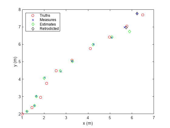
measures = positions + sigmaR*randn(3,steps); Show the truths and measurements in an x-y plot.
figure
plot(positions(1,:),positions(2,:),"ro","DisplayName","Truths");
hold on;
plot(measures(1,:),measures(2,:),"bx","DisplayName","Measures");
xlabel("x (m)")
ylabel("y (m)")
legend("Location","northwest")
Assume that, at the ninth step, the measurement is delayed and therefore unavailable.
delayedMeasure = measures(:,9);
measures(:,9) = NaN;
Construct an extended Kalman filter (EKF) based on the constant velocity model.
estimates = NaN(6,steps);
covariances = NaN(6,6,steps);

estimates(:,1) = positionSelector'*measures(:,1);
covariances(:,:,1) = 1*eye(6);
filter = trackingEKF(@constvel,@cvmeas, ...
    "State",estimates(:,1),...
    "StateCovariance",covariances(:,:,1), ...
    "HasAdditiveProcessNoise",false, ...
    "ProcessNoise",eye(3), ...
    "MeasurementNoise",sigmaR^2*eye(3), ...
    "MaxNumOOSMSteps",3);
Step through the EKF with the measurements.
for ii = 2:steps
    predict(filter);
    if ~any(isnan(measures(:,ii))) % Skip if unavailable
        correct(filter,measures(:,ii));
    end
    estimates(:,ii) = filter.State;
    covariances(:,:,ii) = filter.StateCovariance;
end
Show the estimated results.
plot(estimates(1,:),estimates(3,:),"gd","DisplayName","Estimates");
Retrodict to the ninth step, and correct the current estimates by using the out-of-sequence measurements at the ninth step.
[retroState,retroCov] = retrodict(filter,-1);
[retroCorrState,retroCorrCov] = retroCorrect(filter,delayedMeasure);
Plot the retrodicted state for the ninth step.
plot([retroState(1);retroCorrState(1)],...
     [retroState(3),retroCorrState(3)],...
     "kd","DisplayName","Retrodicted")
You can use the determinant of the final state covariance to see the improvements made by retrodiction. A smaller covariance determinant indicates improved state estimates.
detWithoutRetrodiciton = det(covariances(:,:,end))
detWithoutRetrodiciton =
8.5281e-06
detWithRetrodiciton = det(retroCorrCov)
detWithRetrodiciton =
7.9590e-06
Consider a target moving with a constant velocity model. The initial position is at [100; 0 ;1] in meters. The velocity is [1; 1; 0] in meters per second.
rng(2022) % For repeatable results
initialPosition = [100; 0; 1];
velocity = [1; 1; 0];
Assume the measurement noise covariance matrix is
measureCovaraince = diag([1; 1; 0.1]);
Generate a measurement every second for a duration of five seconds.
measurements = NaN(3,5);
dt = 1;
for i =1:5
    measurements(:,i) = initialPosition + i*dt*velocity + sqrt(measureCovaraince)*randn(3,1);
end
Assume the measurement at the fourth second is out-of-sequence. It only becomes available after the fifth second.
oosm = measurements(:,4);
measurements(:,4) = NaN;
Create a trackingIMM filter with the true initial position using the initekfimm function. Set the maximum number of OOSM steps to five.
detection = objectDetection(0,initialPosition);
imm = initekfimm(detection);
imm.MaxNumOOSMSteps = 5;
Update the filter with the available measurements.
for i = 1:5
    predict(imm,dt);
    if ~isnan(measurements(:,i))
    correct(imm,measurements(:,i));
    end
end
Display the current state, diagonal of state covariance, and model probabilities.
disp("===============Before Retrodiction===============")===============Before Retrodiction===============
disp("Current state:" + newline + num2str(imm.State'))Current state: 106.7626 1.56623 6.15405 1.233862 1.000669 -0.1441939
disp("Diagonal elements of state covariance:" + newline + num2str(diag(imm.StateCovariance)'))Diagonal elements of state covariance: 0.91884 1.1404 0.91861 1.2097 0.91569 1.1156
disp("Model probabities:" + newline + num2str(imm.ModelProbabilities'))Model probabities: 0.51519 0.0016296 0.48318
Retrodict the filter and retrocorrect the filter with the OOSM.
[retroState, retroCov] = retrodict(imm,-1);
retroCorrect(imm,oosm);
Display the results after retrodiction. From the results, the magnitude of state covariance is reduced after the OOSM is applied, showing that retrodiction using OOSM can improve the estimates.
disp("===============After Retrodiction===============")===============After Retrodiction===============
disp("Current state:" + newline + num2str(imm.State'))Current state: 106.6937 1.621093 6.124384 1.261032 1.117407 -0.2363415
disp("Diagonal elements of state covariance:" + newline + num2str(diag(imm.StateCovariance)'))Diagonal elements of state covariance: 0.80678 1.0429 0.81196 1.0962 0.80353 1.0231
disp("Model probabities:" + newline + num2str(imm.ModelProbabilities'))Model probabities: 0.5191 0.00034574 0.48055
Input Arguments
Output Arguments
More About
References
[1] Bar-Shalom, Y., Huimin Chen, and M. Mallick. “One-Step Solution for the Multistep out-of-Sequence-Measurement Problem in Tracking.” IEEE Transactions on Aerospace and Electronic Systems 40, no. 1 (January 2004): 27–37.
[2] Bar-shalom, Y. and Huimin Chen. “IMM Estimator with Out-of-Sequence Measurements.” IEEE Transactions on Aerospace and Electronic Systems, vol. 41, no. 1, Jan. 2005, pp. 90–98.
Extended Capabilities
Version History
Introduced in R2021b