Automatically Tune Filter to Track Maneuvering Targets
This example shows how to tune a tracking filter to track maneuvering targets. It follows up on the Automatically Tune Tracking Filter for Multi-Object Tracker example, which shows how to automatically tune a filter to track non-maneuvering targets. The targets in this example, however, are maneuvering and thus a trackingIMM filter is more suitable for tracking them.
Introduction
Tracking multiple maneuvering targets that move at different speeds and can maneuver very quickly is a challenge. The challenge is further exacerbated when the radar produces false alarms, which may be confused with the real targets. To be able to track such targets, a multi-target tracker must use a well-tuned filter, which tracks each target during both the maneuvering and non-maneuvering sections of its motion.
Having a well-tuned filter is a necessary, but not sufficient, condition. Tracking multiple targets also requires a good association of detections to tracks. Additionally, if the radar provides false alarms, the tracker must distinguish between tracks of real targets and spurious tracks created by the erroneous association of false alarms.
For more information on how to tune a tracker, see the Tuning a Multi-Object Tracker example.
Scenario
The example uses the trajectories described in [1] and implemented in the Benchmark Trajectories for Multi-Object Tracking example. The example creates a scenario with platforms that follow these trajectories. A fusionRadarSensor located at the origin of the scenario frame detects the platforms. Running the scenario produces a recording, which is used to produce the following data:
scans— A structure array that contains the simulation time, platform poses, and detections collected during a single radar sweep across the scenario.truth— A cell array. Each cell contains a timetable with position and velocity information for one truth object.detections— A cell array. Each cell contains a history of all the detections of one truth object.
For brevity, this example loads the needed data from a file, but you can recreate the scenario, detections, truth, and scans using the helperCreateTuningScenario file attached to this example.
load("TuningIMMData.mat","scenario","scans","detections","truth");
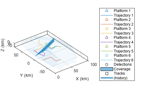
The following line of code creates a visualization object and plots the scenario.
visualization = helperTuningPlotter(scenario);
Track with Untuned Filter
To better understand the challenge in tracking maneuvering targets, create a tracker with an untuned filter. The helperInitLPNHPN function attached to this example initializes a trackingIMM filter with two models. Both models assume that the targets move according to a constant velocity model. The difference between the models is in the process noise level. The low process noise (LPN) filter expects the target to not maneuver and closely follow the constant velocity model. The high process noise (HPN) model allows the target to deviate from the constant velocity model, as it does during maneuvers. Using an interacting multiple model filter with LPN/HPN constant velocity models is common in literature. Here, the process noise of the LPN filter is unit and the variance of the process noise of the HPN filter is 100.
Set the tracker to track no more than 25 targets from a single sensor with the LPN/HPN filter. Increase the confirmation threshold to 4-out-of-5, instead of the 2-out-of-3, to avoid false tracks.
tracker = trackerGNN(MaxNumTracks=25,MaxNumSensors=1, ...
    FilterInitializationFcn=@helperInitLPNHPN, ...
    ConfirmationThreshold=[4 5]);
You control the association of detections to tracks using the AssignmentThreshold property. By default, the control below uses the value of 100, which is also used for the tuned filter later in the example. Adjust the control to see how the AssignmentThreshold value affects the number of track breaks and the metric below.
tracker.AssignmentThreshold =  100;
100;The following line runs the tracker using the radar detections and updates the visualization. The returned value is the result of the optimal sub-pattern association (OSPA) metric configured to compare sets of tracks with sets of truth trajectories, also known as OSPA-on-OSPA or OSPA(2). For more information, see trackOSPAMetric.
untunedOSPA = runTracker(scans,tracker,visualization);
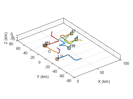
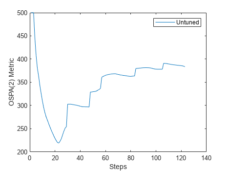
The plot below depicts the OSPA(2) metric. With OSPA, lower values mean better tracking. The plot shows that initially the tracker begins with a good tracking of all targets, but the tracks break when the targets perform sharp maneuvers. Track breaks cause the OSPA(2) metric value to jump.
Tracking can be improved by increasing the AssignmentThreshold property, but high threshold values may lead to more falsely assigned detections and eventually to more falsely confirmed tracks. Explore this by adjusting the AssignmentThreshold slider above.
f = figure;
plot(untunedOSPA,DisplayName="Untuned");
hold on;
xlabel("Steps");
ylabel("OSPA(2) Metric");
legend
Tune Filter
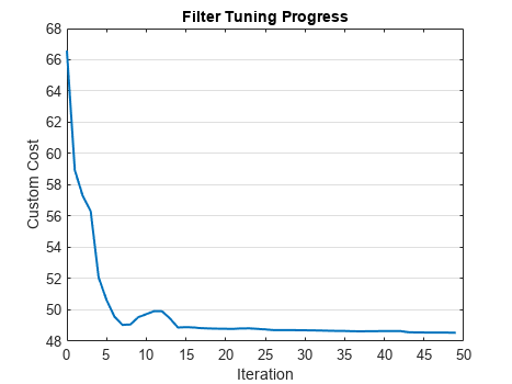
The trackingFilterTuner allows automatic tuning of the filter. Configure the filter to use the same filter initialization function as the tracker and display the tuning progress using a plot.
tuner = trackingFilterTuner(FilterInitializationFcn="helperInitLPNHPN", ...
    Display="Plot");
Choose Tuning Cost
The goal in this example is to tune a filter for multi-target tracking. By choosing to minimize the same cost as the assignment cost, the tuner can tune the filter best for assignment. Therefore, use the helperCostNormalized function attached to this example.
tuner.Cost = "Custom";
tuner.CustomCostFcn = @(trkHistory,truth) helperCostNormalized(trkHistory,truth,"constvel");
Before tuning, compute the untuned filter cost. The cost will be compared with the cost during the tuning process in the next steps. To run the tuner faster, down sample the truth information by a factor of 100.
truth100 = downsample(truth,100);
untunedCost = parameterCost(tuner,[],detections,truth100);
disp("Untuned cost: " + untunedCost);
Untuned cost: 66.0956
Choose Tuned Parameters
The trackingIMM filter contains one filter per model and properties that control how the models interact. By default, the tunable properties of trackingIMM are the TransitionProbabilities and ModelProbabilities properties as well as the tunable filter properties of each tracking filter contained in it. You can click on the links in the display (in live script) to display the tunable filter properties of each tracking filter.
filter = helperInitLPNHPN(detections{1}{1});
tfp = tunableProperties(filter);
disp(tfp);
Tunable properties for object of type: trackingIMM
Property: TransitionProbabilities
PropertyValue: [0.9 0.1;0.1 0.9]
TunedQuantity: Rows sum to one
IsTuned: true
TunedQuantityValue: [0.9 0.1;0.1 0.9]
TunableElements: [1 2 3 4]
LowerBound: [0.001 0.001 0.001 0.001]
UpperBound: [1 1 1 1]
Property: ModelProbabilities
PropertyValue: [0.5;0.5]
TunedQuantity: Columns sum to one
IsTuned: true
TunedQuantityValue: [0.5;0.5]
TunableElements: [1 2]
LowerBound: [0.001 0.001]
UpperBound: [1 1]
The filter contains 2 tracking filters
Show tunable properties for filter 1
Show tunable properties for filter 2
To tune all the tunable filter properties, you enable their tuning using the code section below. Note that tuning more filter properties increases the size of the vector that is being optimized, but potentially can lead to a better overall result. If the tuning takes too long, disable some of the tunable properties.
for i = 1:numel(filter.TrackingFilters)
    setPropertyTunability(tfp,"ProcessNoise","FilterIndex",i,"IsTuned",true);
    setPropertyTunability(tfp,"StateCovariance","FilterIndex",i,"IsTuned",true);
end
tuner.TunablePropertiesSource = "Custom";
tuner.CustomTunableProperties = tfp;
Accelerate Tuning Process
To run the tuning faster, enable both mex and parallel processing.
tuner.UseMex =true; % Requires a MATLAB Coder license tuner.UseParallel =
true; % Requires a Parallel Computing Toolbox license
Run Tuner
Choose the tuner solver algorithm, tune the filter, and observe the improvement in cost in the graph.
When choosing the solver, use "active-set" if you do not have a license to Optimization Toolbox or Global Optimization Toolbox.
tuner.Solver = "fmincon";
tic;
[tunedParameters,tunedCost] = tune(tuner,detections,truth100);
"fmincon";
tic;
[tunedParameters,tunedCost] = tune(tuner,detections,truth100);Generating code. Code generation successful.
disp("Time it took to tune the IMM filter: " + toc + " seconds");
Time it took to tune the IMM filter: 169.0394 seconds
Analyze Tuning Results
You can use the plotFilterErrors object function to analyze if the filter is unbiased and consistent. If the errors average around zero, the filter is unbiased. If the errors are contained within the 3-sigma band in most of the steps, the filter is consistent. The following plot shows that both criteria are satisfied, which is a sign of good tuning.
plotFilterErrors(tuner);
![Figure Filter estimate error contains 6 axes objects. Axes object 1 with xlabel Time [sec], ylabel X_{Error} contains 12 objects of type line, patch. Axes object 2 with xlabel Time [sec], ylabel V_X_{Error} contains 12 objects of type line, patch. Axes object 3 with xlabel Time [sec], ylabel Y_{Error} contains 12 objects of type line, patch. Axes object 4 with xlabel Time [sec], ylabel V_Y_{Error} contains 12 objects of type line, patch. Axes object 5 with xlabel Time [sec], ylabel Z_{Error} contains 12 objects of type line, patch. Axes object 6 with xlabel Time [sec], ylabel V_Z_{Error} contains 12 objects of type line, patch. These objects represent Realizations, 3\sigma.](../../examples/fusion/win64/TuneIMMFilterExample_05.png)
Observe the filter interactivity properties. The TransitionProbabilities property defines how likely the models are to not switch (main diagonal) versus to switch (off-diagonal values). Main diagonal values are expected to be higher than off-diagonal ones. Otherwise, the filter may flip between the models too easily.
disp(tunedParameters.TransitionProbabilities)
    0.9729    0.0271
    0.0282    0.9718
The ModelProbabilities property shows the probability of each model when the filter is initialized. The expected values are around 50-50, which is also the default. You can leave this property untuned, but the results show that the probability of the HPN filter is slightly higher than the probability of the LPN filter.
disp(tunedParameters.ModelProbabilities);
    0.4148
    0.5852
The process noises of both filters should indicate the highest unknown maneuver acceleration they allow. To evaluate that, first compute the eigenvalues of the process noise, which indicates the variance value, then take the square root to get the standard deviation. The division by the value of g is to compute the highest number of "G's" the filter expects the target to take. Reference [1] indicates that the maneuvers are up to 7G turns, which is close to what the tuned filter allows.
g = 9.81;
disp(sqrt(norm(eig(tunedParameters.TrackingFilters{1}.ProcessNoise)))/g);
0.4688
disp(sqrt(norm(eig(tunedParameters.TrackingFilters{2}.ProcessNoise)))/g);6.3047
Track with Tuned Filter
A tuned filter is necessary for a good multi-target tracking, but it is still not guaranteed that the tracking is good. To check it, use the exportToFunction object function to get the tuned filter initialization function.
exportToFunction(tuner,"tunedInitFcn");Use the tuned filter initialization function in the tracker and rerun the tracker, then plot the values of the tuned OSPA(2) metric.
release(tracker);
tracker.FilterInitializationFcn = @tunedInitFcn;
tunedOSPA = runTracker(scans,tracker,visualization);

![Figure Filter estimate error contains 6 axes objects. Axes object 1 with xlabel Time [sec], ylabel X_{Error} contains 12 objects of type line, patch. Axes object 2 with xlabel Time [sec], ylabel V_X_{Error} contains 12 objects of type line, patch. Axes object 3 with xlabel Time [sec], ylabel Y_{Error} contains 12 objects of type line, patch. Axes object 4 with xlabel Time [sec], ylabel V_Y_{Error} contains 12 objects of type line, patch. Axes object 5 with xlabel Time [sec], ylabel Z_{Error} contains 12 objects of type line, patch. Axes object 6 with xlabel Time [sec], ylabel V_Z_{Error} contains 12 objects of type line, patch. These objects represent Realizations, 3\sigma.](../../examples/fusion/win64/TuneIMMFilterExample_07.png)
The tuned OSPA(2) value is much lower than the untuned value, which indicates better tracking. The lack of "jumps" in the tuned metric also indicates that there were no undesired track switches, drops, or false tracks.
plot(gca(figure(f)),tunedOSPA,DisplayName="Tuned");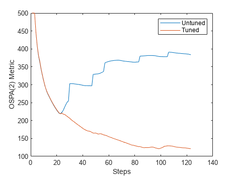
Summary
This example showed how to tune an interacting multiple model (IMM) filter and use it in a multi-target tracker to track highly maneuvering targets. The tuned filter allows the tracker to have a tight assignment gate and the OSPA(2) metric showed that there were no track switches or breaks even when the targets maneuvered. Finally, setting the confirmation threshold to a higher value prevented the tracker from confirming false tracks.
References
[1] W.D. Blair, G. A. Watson, T. Kirubarajan, Y. Bar-Shalom, "Benchmark for Radar Allocation and Tracking in ECM." Aerospace and Electronic Systems IEEE Trans on, vol. 34. no. 4. 1998
function metricValues = runTracker(scans,tracker,visualization)
reset(visualization);
reset(tracker);
metric = trackOSPAMetric(Metric="OSPA(2)",Distance="posabserr",CutoffDistance=500);
metricValues = zeros(1,numel(scans));

for i = 1:numel(scans)
    time = scans(i).Time;
    poses = scans(i).Poses;
    detections = scans(i).Detections;

    tracks = tracker(detections, time);
    metricValues(i) = metric(tracks,poses);

    update(visualization,poses(1:6),detections,tracks);
end
end