Adaptive Noise Cancellation Using ANFIS

This example shows how to do adaptive nonlinear noise cancellation by constructing and tuning an ANFIS model.

Signal and Noise

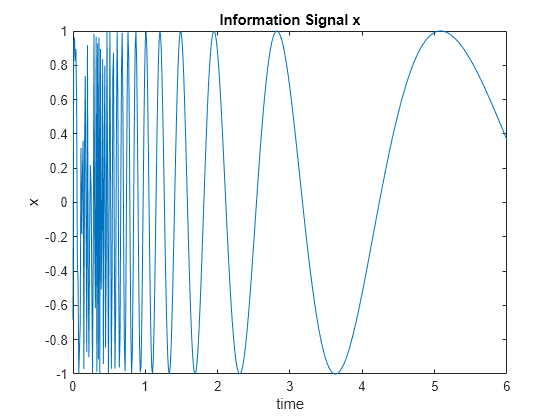
Define a hypothetical information signal, x, sampled at 100 Hz over 6 seconds.

time = (0:0.01:6)';
x = sin(40./(time+0.01));
plot(time,x)
title('Information Signal x')
xlabel('time')
ylabel('x')

Assume that x cannot be measured without an interference signal, ${\mathit{n}}_2$, which is generated from another noise source, ${\mathit{n}}_1$, by a certain unknown nonlinear process.

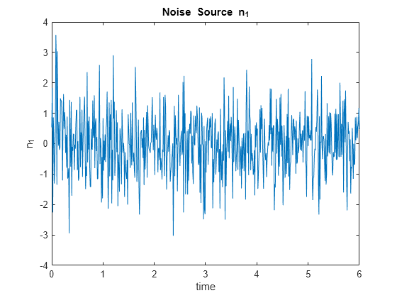
Generate and plot the noise source ${\mathit{n}}_1$.

n1 = randn(size(time));
plot(time,n1)
title('Noise Source n_1')
xlabel('time')
ylabel('n_1')

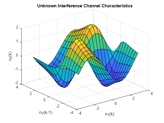
Assume that the interference signal, ${\mathit{n}}_2$, that appears in the measured signal is generated via an unknown nonlinear equation:

$$n_2\left(k\right)=\frac{4\sin \left(n_1\left(k\right)\right)\cdot n_1\left(k-1\right)}{1+n_1{\left(k-1\right)}^2}$$

Plot this nonlinear function as a surface.

domain = linspace(min(n1),max(n1),20);
[xx,yy] = meshgrid(domain,domain);
zz = 4*sin(xx).*yy./(1+yy.^2);

surf(xx,yy,zz)
xlabel('n_1(k)')
ylabel('n_1(k-1)')
zlabel('n_2(k)')
title('Unknown Interference Channel Characteristics')

Compute the interference signal, ${\mathit{n}}_2$, from the noise source, ${\mathit{n}}_1$, and plot both signals.

n1d0 = n1;                            % n1 with delay 0
n1d1 = [0; n1d0(1:length(n1d0)-1)];   % n1 with delay 1
n2 = 4*sin(n1d0).*n1d1./(1+n1d1.^2);  % interference

subplot(2,1,1)
plot(time,n1)
ylabel('n_1')
xlabel('time')
title('Noise Source')
subplot(2,1,2)
plot(time,n2)
ylabel('n_2')
title('Interference Signal')
xlabel('time')

${\mathit{n}}_2$ is related to ${\mathit{n}}_1$ by the highly nonlinear process shown previously. However, from the plots, these two signals do not appear to correlate with each other in any way.

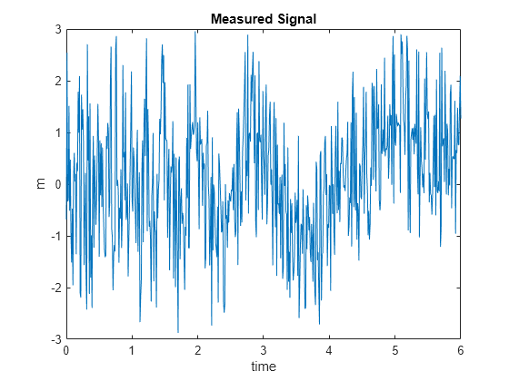
The measured signal, m, is the sum of the original information signal, x, and the interference, ${\mathit{n}}_2$. However, ${\mathit{n}}_2$ is unknown. The only available signals are the noise signal, ${\mathit{n}}_1$, and the measured signal m.

m = x + n2;
subplot(1,1,1)
plot(time, m)
title('Measured Signal')
xlabel('time')
ylabel('m')

You can recover the original information signal, x, using adaptive noise cancellation via ANFIS training.

Build the ANFIS Model

Use the anfis command to identify the nonlinear relationship between ${\mathit{n}}_1$ and ${\mathit{n}}_2$. While ${\mathit{n}}_2$ is not directly available, you can assume that m is a noisy version of ${\mathit{n}}_2$ for training. This assumption treats x as "noise" in this kind of nonlinear fitting.

Assume the order of the nonlinear channel is known (in this case, 2). You can use a two-input ANFIS model for training.

Define the training data. The first two columns of data are the inputs to the ANFIS model, ${\mathit{n}}_1$ and a delayed version of ${\mathit{n}}_1$. The final column of data is the measured signal, m.

delayed_n1 = [0; n1(1:length(n1)-1)];
data = [delayed_n1 n1 m];

Generate the initial FIS object. By default, the grid partitioning algorithm uses two membership functions for each input variable, which produces four fuzzy rules for learning.

genOpt = genfisOptions('GridPartition');
inFIS = genfis(data(:,1:end-1),data(:,end),genOpt);

Tune the FIS using the anfis command with an initial training step size of 0.2.

trainOpt = anfisOptions('InitialFIS',inFIS,'InitialStepSize',0.2);
outFIS = anfis(data,trainOpt);

ANFIS info:
	Number of nodes: 21
	Number of linear parameters: 12
	Number of nonlinear parameters: 12
	Total number of parameters: 24
	Number of training data pairs: 601
	Number of checking data pairs: 0
	Number of fuzzy rules: 4


Start training ANFIS ...

1 	 0.761817
2 	 0.748426
3 	 0.739315
4 	 0.733993
Step size increases to 0.220000 after epoch 5.
5 	 0.729492
6 	 0.725382
7 	 0.721269
8 	 0.717621
Step size increases to 0.242000 after epoch 9.
9 	 0.714474
10 	 0.71207

Designated epoch number reached. ANFIS training completed at epoch 10.

Minimal training RMSE = 0.71207

The tuned FIS, outFIS, models the second-order relationship between ${\mathit{n}}_1$ and ${\mathit{n}}_2$.

Evaluate Model

Calculate the estimated interference signal, estimated_n2, by evaluating the tuned FIS using the original training data.

estimated_n2 = evalfis(outFIS,data(:,1:2));

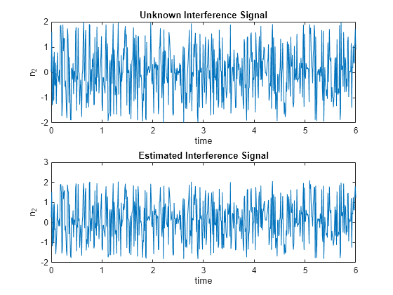
Plot the actual ${\mathit{n}}_2$ signal and the estimated version from the ANFIS output.

subplot(2,1,1)
plot(time, n2)
ylabel('n_2')
xlabel('time')
title('Unknown Interference Signal')
subplot(2,1,2)
plot(time, estimated_n2)
ylabel('n_2')
xlabel('time')
title('Estimated Interference Signal')

The estimated information signal is equal to the difference between the measured signal, m, and the estimated interference (ANFIS output).

estimated_x = m - estimated_n2;

Compare the original information signal, x, and the estimate, estimated_x.

figure
plot(time,estimated_x,'b',time,x,'r')
xlabel('time')
ylabel('x')
title('Comparison of Actual and Estimated Signals')
legend('Estimated x','Actual x (unknown)','Location','SouthEast')

Without extensive training, the ANFIS model produces a relatively accurate estimate of the information signal.