Main Content

era

Estimate state-space model from impulse response data using Eigensystem Realization Algorithm (ERA)

Since R2022b

Description

era uses the Eigensystem Realization Algorithm [1] to estimate a state-space model using impulse response data rather than input/output data. era is especially useful for identifying dynamic systems for applications such as modal analysis or structural health modeling. You can also use era for modeling time-series data for applications such as prediction. For more information about the algorithm, see [1].

example

sys = era(data) estimates a state-space model using the time-domain impulse response data in data, which can be either a timetable or matrix that contains only output data. The software determines the order of the model nx automatically.

sys is a model of the following form:

x˙(t)=Ax(t)+Bu(t)+Ke(t)y(t)=Cx(t)+Du(t)+e(t)

A, B, C, D, and K are state-space matrices. u(t) is the input, y(t) is the output, e(t) is the disturbance, and x(t) is the vector of nx states.

All entries of A, B, C, and K are free estimable parameters by default. D is fixed to zero by default, meaning that there is no feedthrough, except for static systems (nx = 0).

The software sets the sample time of sys to the sample time of data if data is a timetable, or to -1 if data is a matrix.

example

sys = era(data,nx) specifies the number of states nx.

example

sys = era(data,nx,Name=Value) incorporates additional options specified by one or more name-value arguments. For example, use the Feedthrough name-value argument to introduce feedthrough by estimating the D matrix. Use the InputDelay name-value argument to specify input delays for each channel.

Examples

collapse all

Load and plot the data Htt, which is a timetable that contains impulse response data in the variable H.

load impulseresponse.mat Htt
plot(Htt.Time,Htt.H)
title('Impulse Response')

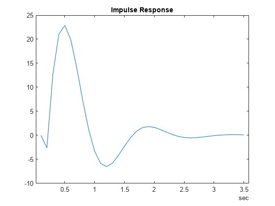
Use era to estimate a state-space model.

sys = era(Htt);
sysorder = order(sys)
sysorder = 2

sys is an idss model of order 2.

Load and plot the data H, which is a numeric matrix. Ts is the sample time for the data in H.

load impulseresponse.mat H Ts
L = size(H,1);
t = (1:L)'*Ts;
plot(t,H)
title('Impulse Response')

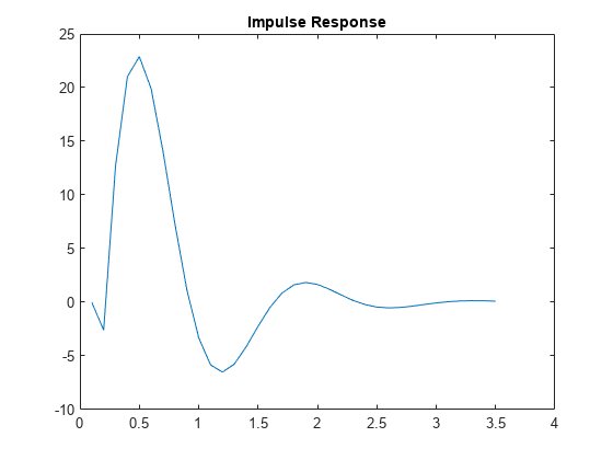
Use era to estimate a state-space model of order 3.

sys = era(H,3);
sysorder = order(sys)
sysorder = 3

sys is an idss model of order 3.

Load the impulse response data, which is in the form of a timetable.

load impulseresponse.mat Htt

Use era to specify a state-space model that includes feedthrough.

sys = era(Htt,'best',Feedthrough=1);

Input Arguments

collapse all

Impulse response data, specified as either a timetable with Ns rows and Ny variables or an Ns-by-Ny-by-Nu numeric matrix, where Ns is the number of samples, Ny is the number of outputs, and Nu is the number of inputs. data must be uniformly sampled.

  • For SISO and SIMO systems, each column i of the timetable or matrix in data represents the impulse response from the single input to the ith output.

  • For MIMO systems, data must be a 3-D matrix. Each Ns-length vector (i,j) of data represents the impulse response between output i and input j, data(:,i,j).

data must be obtained from a system with zero initial conditions.

Order of the estimated model, specified as a nonnegative integer, a vector containing a range of positive integers, or "best".

  • If you already know what order you want your estimated model to have, specify nx as a scalar.

  • If you want to compare a range of potential orders to choose the most effective order for your estimated model, specify the range in nx. era creates a Hankel singular-value plot that shows the relative energy contributions of each state in the system. States with relatively small Hankel singular values contribute little to the accuracy of the model and can be discarded with little impact. The index of the highest state you retain is the model order. The plot window includes a suggestion for the order to use. You can accept this suggestion or enter a different order. For an example of using Hankel plots, see ssest.

    If you do not specify nx or if you specify nx as "best", the software automatically chooses nx from the range 1:10.

  • If you are identifying a static system, set nx to 0.

Name-Value Arguments

Specify optional pairs of arguments as Name1=Value1,...,NameN=ValueN, where Name is the argument name and Value is the corresponding value. Name-value arguments must appear after other arguments, but the order of the pairs does not matter.

Example: sys = era(data,2,InputDelay=1)

Input delay for each input channel, specified as a numeric vector of length equal to the number of inputs in sys. To apply the same delay to all channels, specify InputDelay as a numeric scalar.

Option to include direct feedthrough from input to output, specified as a logical vector of length Nu, where Nu is the number of inputs. If you specify Feedthrough as a logical scalar, that value is applied to all the inputs. The default is 0, except for static systems, where the software always assumes Feedthrough is 1.

Output Arguments

collapse all

Identified state-space model, returned as an idss array for SISO systems or, for systems with more than one input or output, an array of idss models. Each model represents the response of one input to one output. This model is created using the specified model order and delays.

Information about the estimation results and options used is stored in the Report property of the model. Report has the same fields as an idss model that was generated using estimation commands such as ssest. However, models generated with era do not use all these fields.

Report FieldDescription
Status

For era-based models, Estimated using the Eigensystem Realization Algorithm

Method

ERA

FitQuantitative assessment of the estimation, returned as a structure
Parameters

Estimated values of model parameters

OptionsUsed

[]

RandState[]
DataUsedAttributes of the data used for estimation
Termination[]

For more information on using Report, see Estimation Report.

References

[1] Juang, Jer-Nan, and Richard S. Pappa. “An Eigensystem Realization Algorithm for Modal Parameter Identification and Model Reduction.” Journal of Guidance, Control, and Dynamics 8, no. 5 (September 1985): 620–27. https://doi.org/10.2514/3.20031.

Version History

Introduced in R2022b