Analyze Hyperspectral and Multispectral Images

Hyperspectral and multispectral imaging are advanced techniques to capture and analyze the spectral information of objects across various wavelengths. Hyperspectral imaging collects data in numerous narrow and contiguous spectral bands, often exceeding 100, providing detailed spectral fingerprints that enable precise material identification and discrimination. This makes it particularly useful for applications such as mineralogy and environmental monitoring. Hyperspectral imaging is also useful in non-destructive testing applications in manufacturing. In medical imaging, you can use hyperspectral images to identify types of tissue or to detect abnormalities based on spectral signature. On the other hand, multispectral imaging captures data in fewer, broader bands, typically ranging from 3 to 10. While multispectral imaging offers less spectral detail than hyperspectral imaging, it is efficient and effective for applications such as land cover classification. You can also use multispectral imaging in agriculture by installing multispectral cameras on drones and analyzing reflectance in different spectral bands to assess crop health. Both techniques play crucial roles in scientific and industrial applications such as remote sensing and medical imaging, enabling enhanced analysis and decision-making based on spectral data.

This example requires the Hyperspectral Imaging Library for Image Processing Toolbox™. You can install the Hyperspectral Imaging Library for Image Processing Toolbox from Add-On Explorer. For more information about installing add-ons, see Get and Manage Add-Ons. The Hyperspectral Imaging Library for Image Processing Toolbox requires desktop MATLAB^®, as MATLAB Online™ and MATLAB Mobile™ do not support the library.

Hyperspectral Image Analysis

The Hyperspectral Imaging Library for Image Processing Toolbox provides several functionalities for hyperspectral image processing. You can import hyperspectral data into the workspace as a hypercube object. You can create a hypercube object from imported data acquired using one of these methods.

Data acquired by these satellites:
- EO-1 Hyperion
- Airborne Visible/Infrared Imaging Spectrometer (AVIRIS)
Spectral data cube with uniform resolution across all spectral bands.
Spectral data from file types supported by imhypercube and geohypercube.

You can create a hypercube object using the imhypercube or geohypercube function.

Use the imhypercube function when you do not require the geospatial information for your application. For example, applications of hyperspectral data such as non-destructive testing, medical imaging, or local land cover assessment do not require geospatial information for the acquired data.
Use the geohypercube function for remote sensing applications when you have geospatial information for the data, such as the geographic location, spatial referencing information, and its projected coordinates system. The geospatial information enables you to map an analysis such as environmental monitoring, to geographic coordinates. The geohypercube function requires a Mapping Toolbox™ license.

Analyze Hyperspectral Image With and Without Geospatial Information

This example uses:

Open Live Script

This example uses hyperspectral data acquired by the Airborne Visible Infrared Imaging Spectrometer (AVIRIS) and made publicly available for use by NASA/JPL-Caltech. Download and unzip the data set. The total size of the data set is approximately 7GB. The download might take a long time depending on your internet connection.

zipFile = matlab.internal.examples.downloadSupportFile("image","data/f140826t01p00r08rdn_b.zip");
filepath = fileparts(zipFile);
unzip(zipFile,filepath)
filename = fullfile(filepath,"f140826t01p00r08rdn_b","f140826t01p00r08rdn_b_sc01_ort_img");

Load the hyperspectral data into the workspace without geospatial information. Note that the size of the hyperspectral image is 27068-by-1302-by-224, which would require a large amount of system memory to process at once. Crop the hyperspectral image to get a 50-by-50-by-100 hyperspectral image.

hcube = imhypercube(filename);
hcube.ImageDims

ans = 
"[27068x1302x224 int16]"

hcube = cropData(hcube,22951:23000,501:550,1:100);
hcube.ImageDims

ans = 
"[50x50x100 int16]"

Visualize an estimated RGB image of the cropped hyperspectral data.

rgbImg = colorize(hcube,Method="rgb",ContrastStretching=true);
figure
imageshow(rgbImg)

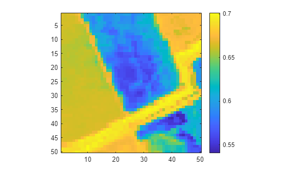
Compute and visualize the spectral matching score for the cropped hyperspectral data with the spectral signature for vegetation. Observe that a score of 0.63 or lower indicates vegetation.

vegSigFile = "vegetation.tree.tsuga.canadensis.vswir.tsca-1-47.ucsb.asd.spectrum.txt";
vegLibData = readEcostressSig(vegSigFile);
vegScore = spectralMatch(vegLibData,hcube);
figure
imagesc(vegScore)
axis equal tight
colorbar

Observe that the imported hyperspectral data does not have any geospatial information. Thus, you cannot map the spectral analysis to geographic coordinates.

R = hcube.Metadata.RasterReference

R =

     []

To map the spectral analysis to geographic coordinates, load the hyperspectral data into the workspace with its geospatial information, and repeat the analysis.

hcube = geohypercube(filename);
hcube = cropData(hcube,22951:23000,501:550,1:100);
vegScore = spectralMatch(vegLibData,hcube);

Create a polygonal region of interest in geographic coordinates.

R = hcube.Metadata.RasterReference

R = 
  MapCellsReference with properties:

            XWorldLimits: [621542.421533526 622592.045803597]
            YWorldLimits: [3659016.39601544 3660066.02028551]
              RasterSize: [50 50]
    RasterInterpretation: 'cells'
        ColumnsStartFrom: 'north'
           RowsStartFrom: 'west'
      CellExtentInWorldX: 15.9
      CellExtentInWorldY: 15.9
    RasterExtentInWorldX: 795
    RasterExtentInWorldY: 795
        XIntrinsicLimits: [0.5 50.5]
        YIntrinsicLimits: [0.5 50.5]
      TransformationType: 'affine'
    CoordinateSystemType: 'planar'
            ProjectedCRS: [1×1 projcrs]

xlimits = R.XWorldLimits;
ylimits = R.YWorldLimits;
dataRegion = mappolyshape(xlimits([1 1 2 2 1]),ylimits([1 2 2 1 1]));
dataRegion.ProjectedCRS = R.ProjectedCRS;

Obtain the x and y world coordinates of the pixels of the high-vegetation regions in the polyX and polyY cell arrays. Apply a threshold of 0.63 on the spectral matching score to consider only the high-vegetation regions.

[rowsVec,colsVec] = find(vegScore <= 0.63);
[polyX,polyY] = intrinsicToWorld(R,colsVec,rowsVec);

Map the high-vegetation regions to the coordinate system of the hyperspectral data.

shape = mappointshape(polyX,polyY);
shape.ProjectedCRS = R.ProjectedCRS;

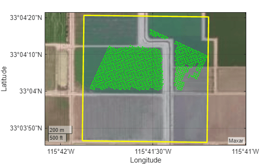
Plot the polygonal region of interest and the high-vegetation regions within the region of interest on satellite imagery.

figure
geoplot(dataRegion, ...
    LineWidth=2, ...
    EdgeColor="yellow", ...
    FaceAlpha=0.2)
hold on
geoplot(shape,"g.")
geobasemap satellite

Multispectral Image Analysis

The Hyperspectral Imaging Library for Image Processing Toolbox provides several functionalities for multispectral image processing. You can import multispectral data into the workspace as a multicube object. You can create a multicube object from imported data acquired using one of these methods.

Data acquired by these satellites:
- EO-1 Advanced Land Imager (EO-1 ALI)
- Landsat Multispectral Scanner (Landsat MSS)
- Landsat Thematic Mapper (Landsat TM)
- Landsat Enhanced Thematic Mapper Plus (Landsat ETM+)
- Landsat Operational Land Imager / Thermal Infrared Scanner (Landsat OLI / TIRS)
Spectral data cube with uniform resolution across all spectral bands.
Spectral data from file types supported by immulticube and geomulticube.

You can create the multicube object using the immulticube or geomulticube function.

Use the immulticube function when you do not require the geospatial information for your application. For example, applications of multispectral data such as local crop health assessment might not require geospatial information for the acquired data.
Use the geomulticube function for remote sensing applications when you have geospatial information for the data, such as the geographic location, spatial referencing information, and its projected coordinates system. The geospatial information enables you to map an analysis, such as land use land cover classification, to geographic coordinates. The geomulticube function requires a Mapping Toolbox license.

Analyze Multispectral Image With and Without Geospatial Information

This example uses:

Open Live Script

This example uses Landsat 8 multispectral data. Download and unzip the data set.

zipfile = "LC08_L1TP_113082_20211206_20211215_02_T1.zip";
landsat8Data_url = "https://ssd.mathworks.com/supportfiles/image/data/" + zipfile;
hyper.internal.downloadLandsatDataset(landsat8Data_url,zipfile)
filename = fullfile("LC08_L1TP_113082_20211206_20211215_02_T1","LC08_L1TP_113082_20211206_20211215_02_T1_MTL.txt");

Load the multispectral data into the workspace without geospatial information. Crop the multispectral data to a smaller size for faster processing.

mcube = immulticube(filename);
mcube = selectBands(mcube,DataResolution=30);
mcube = cropData(mcube,3001:4000,5001:6000);

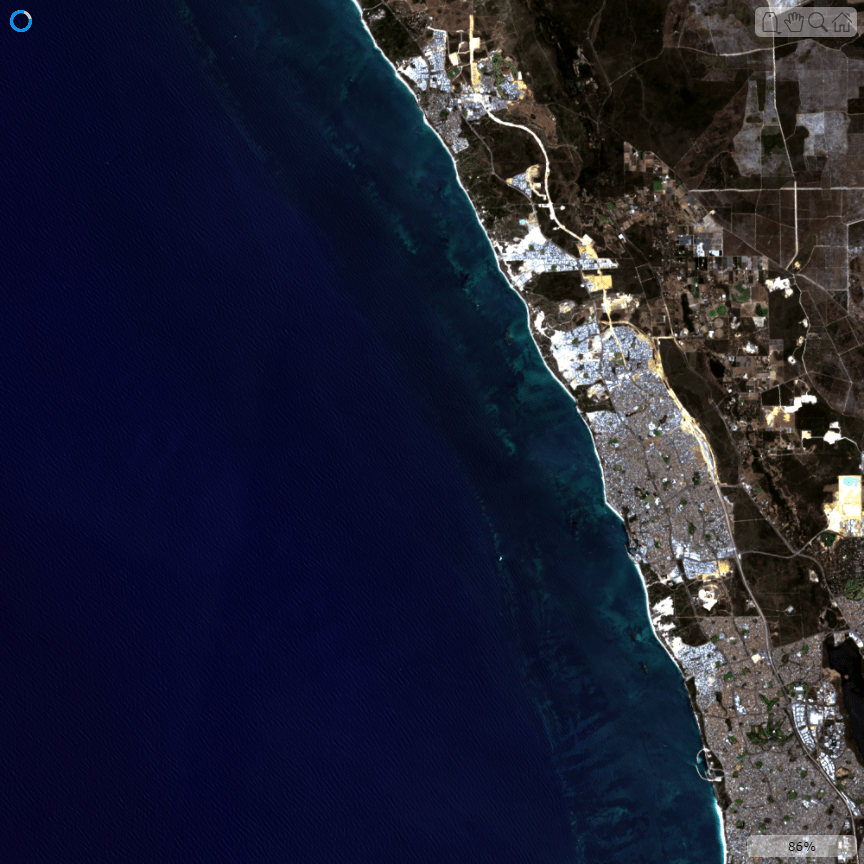
Visualize an estimated RGB image of the cropped multispectral data.

rgbImg = colorize(mcube,ContrastStretching=true);
figure
imageshow(rgbImg)

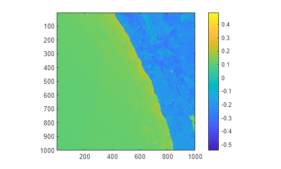
Compute and visualize the spectral index MNDWI for the multispectral data to identify water regions. Observe that an index value of 0.1 or greater indicates water.

mndwi = spectralIndices(mcube,"MNDWI");
mndwiImg = mndwi.IndexImage;
figure
imagesc(mndwiImg)
axis equal tight
colorbar

Observe that the imported multispectral data does not have any geospatial information. Thus, you cannot map the spectral analysis to geographic coordinates.

R = mcube.Metadata.RasterReference

R =

     []

To map the spectral analysis to geographic coordinates, load the multispectral data into the workspace with its geospatial information, and repeat the analysis.

mcube = geomulticube(filename);
mcube = selectBands(mcube,DataResolution=30);
mcube = cropData(mcube,3001:4000,5001:6000);
mndwi = spectralIndices(mcube,"MNDWI");
mndwiImg = mndwi.IndexImage;

Create a polygonal region of interest in geographic coordinates. As the size of the spectral index image is the same as the size of the first band in the multispectral image, use the geospatial information of the first band of the multispectral image.

R = mcube.Metadata.RasterReference

R = 
  10×1 MapPostingsReference array with properties:

    RasterInterpretation
    XIntrinsicLimits
    YIntrinsicLimits
    SampleSpacingInWorldX
    SampleSpacingInWorldY
    XWorldLimits
    YWorldLimits
    RasterSize
    ColumnsStartFrom
    RowsStartFrom
    RasterExtentInWorldX
    RasterExtentInWorldY
    TransformationType
    CoordinateSystemType
    ProjectedCRS

xlimits = R(1).XWorldLimits;
ylimits = R(1).YWorldLimits;
dataRegion = mappolyshape(xlimits([1 1 2 2 1]),ylimits([1 2 2 1 1]));
dataRegion.ProjectedCRS = R(1).ProjectedCRS;

Obtain the x and y world coordinates of the pixels of the water regions in the polyX and polyY cell arrays. Apply a threshold of 0.1 on the spectral matching score to consider only the water regions.

[rowsVec,colsVec] = find(mndwiImg >= 0.1);
[polyX,polyY] = intrinsicToWorld(R(1),colsVec,rowsVec);

Map the water regions to the coordinate system of the multispectral data.

shape = mappointshape(polyX,polyY);
shape.ProjectedCRS = R(1).ProjectedCRS;

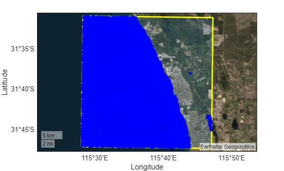
Plot the polygonal region of interest and the water regions within the region of interest on satellite imagery. This process might take a long time depending on your system configuration.

figure
geoplot(dataRegion, ...
    LineWidth=2, ...
    EdgeColor="yellow", ...
    FaceAlpha=0.2)
hold on
geoplot(shape,"b.")
geobasemap satellite