Main Content

Working with Delaunay Triangulations

Definition of Delaunay Triangulation

Delaunay triangulations are widely used in scientific computing in many diverse applications. While there are numerous algorithms for computing triangulations, it is the favorable geometric properties of the Delaunay triangulation that make it so useful.

The fundamental property is the Delaunay criterion. In the case of 2-D triangulations, this is often called the empty circumcircle criterion. For a set of points in 2-D, a Delaunay triangulation of these points ensures the circumcircle associated with each triangle contains no other point in its interior. This property is important. In the illustration below, the circumcircle associated with T1 is empty. It does not contain a point in its interior. The circumcircle associated with T2 is empty. It does not contain a point in its interior. This triangulation is a Delaunay triangulation.

Delaunay triangulation with circumcircles plotted.

The triangles below are different. The circumcircle associated with T1 is not empty. It contains V3 in its interior. The circumcircle associated with T2 is not empty. It contains V1 in its interior. This triangulation is not a Delaunay triangulation.
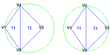
Non-Delaunay triangulation with circumcircles plotted.

Delaunay triangles are said to be “well shaped” because in fulfilling the empty circumcircle property, triangles with large internal angles are selected over ones with small internal angles. The triangles in the non-Delaunay triangulation have sharp angles at vertices V2 and V4. If the edge {V2, V4} were replaced by an edge joining V1 and V3, the minimum angle would be maximized and the triangulation would become a Delaunay triangulation. Also, the Delaunay triangulation connects points in a nearest-neighbor manner. These two characteristics, well-shaped triangles and the nearest-neighbor relation, have important implications in practice and motivate the use of Delaunay triangulations in scattered data interpolation.

While the Delaunay property is well defined, the topology of the triangulation is not unique in the presence of degenerate point sets. In two dimensions, degeneracies arise when four or more unique points lie on the same circle. The vertices of a square, for example, have a nonunique Delaunay triangulation.
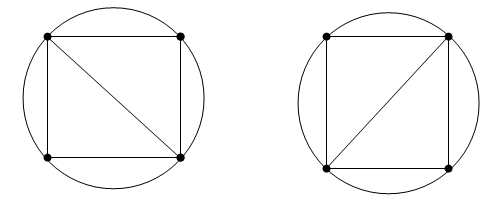
Delaunay triangulation of the vertices of a square, for which two different valid Delaunay triangulations are possible.

The properties of Delaunay triangulations extend to higher dimensions. The triangulation of a 3-D set of points is composed of tetrahedra. The next illustration shows a simple 3-D Delaunay triangulation made up of two tetrahedra. The circumsphere of one tetrahedron is shown to highlight the empty circumsphere criterion.
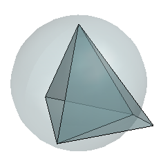
3-D Delaunay triangulation with circumsphere.

A 3-D Delaunay triangulation produces tetrahedra that satisfy the empty circumsphere criterion.

Creating Delaunay Triangulations

MATLAB® provides two ways to create Delaunay triangulations:

The delaunay function supports the creation of 2-D and 3-D Delaunay triangulations. The delaunayn function supports creating Delaunay triangulations in 4-D and higher.

Tip

Creating Delaunay triangulations in dimensions higher than 6-D is generally not practical for moderate to large point sets due to the exponential growth in required memory.

The delaunayTriangulation class supports creating Delaunay triangulations in 2-D and 3-D. It provides many methods that are useful for developing triangulation-based algorithms. These class methods are like functions, but they are restricted to work with triangulations created using delaunayTriangulation. The delaunayTriangulation class also supports the creation of related constructs such as the convex hull and Voronoi diagram. It also supports the creation of constrained Delaunay triangulations.

In summary:

  • The delaunay function is useful when you only require the basic triangulation data, and that data is sufficiently complete for your application.

  • The delaunayTriangulation class offers more functionality for developing triangulation-based applications. It is useful when you require the triangulation and you want to perform any of these operations:

    • Search the triangulation for triangles or tetrahedra enclosing a query point.

    • Use the triangulation to perform a nearest-neighbor point search.

    • Query the triangulation's topological adjacency or geometric properties.

    • Modify the triangulation to insert or remove points.

    • Constrain edges in the triangulation—this is called a constrained Delaunay triangulation.

    • Triangulate a polygon and optionally remove the triangles that are outside of the domain.

    • Use the Delaunay triangulation to compute the convex hull or Voronoi diagram.

Using the delaunay and delaunayn functions

The delaunay and delaunayn functions take a set of points and produce a triangulation in matrix format. Refer to Triangulation Matrix Format for more information on this data structure. In 2-D, the delaunay function is often used to produce a triangulation that can be used to plot a surface defined in terms of a set of scattered data points. In this application, it’s important to note that this approach can only be used if the surface is single-valued. For example, it could not be used to plot a spherical surface because there are two z values corresponding to a single (x, y) coordinate. A simple example demonstrates how the delaunay function can be used to plot a surface representing a sampled data set.

This example shows how to use the delaunay function to create a 2-D Delaunay triangulation from the seamount data set. A seamount is an underwater mountain. The data set consists of a set of longitude (x) and latitude (y) locations, and corresponding seamount elevations (z) measured at those coordinates.

Load the seamount data set and view the (x, y) data as a scatter plot.

load seamount
plot(x,y,'.','markersize',12)
xlabel('Longitude'), ylabel('Latitude')
grid on

Figure contains an axes object. The axes object with xlabel Longitude, ylabel Latitude contains a line object which displays its values using only markers.

Construct a Delaunay triangulation from this point set and use triplot to plot the triangulation in the existing figure.

tri = delaunay(x,y);
hold on, triplot(tri,x,y), hold off

Figure contains an axes object. The axes object with xlabel Longitude, ylabel Latitude contains 2 objects of type line. One or more of the lines displays its values using only markers

Add the depth data (z) from seamount to lift the vertices and create the surface. Create a new figure and use trimesh to plot the surface in wireframe mode.

figure
hidden on
trimesh(tri,x,y,z)
xlabel('Longitude'),ylabel('Latitude'),zlabel('Depth in Feet');

Figure contains an axes object. The axes object with xlabel Longitude, ylabel Latitude contains an object of type patch.

If you want to plot the surface in shaded mode, use trisurf instead of trimesh.

A 3-D Delaunay triangulation also can be created using the delaunay function. This triangulation is composed of tetrahedra.

This example shows how to create a 3-D Delaunay triangulation of a random data set. The triangulation is plotted using tetramesh, and the FaceAlpha option adds transparency to the plot.

rng('default')
X = rand([30 3]);
tet = delaunay(X);
faceColor  = [0.6875 0.8750 0.8984];
tetramesh(tet,X,'FaceColor', faceColor,'FaceAlpha',0.3);

Figure contains an axes object. The axes object contains 102 objects of type patch.

MATLAB provides the delaunayn function to support the creation of Delaunay triangulations in dimension 4-D and higher. Two complementary functions tsearchn and dsearchn are also provided to support spatial searching for N-D triangulations. See Spatial Searching for more information on triangulation-based search.

Using the delaunayTriangulation Class

The delaunayTriangulation class provides another way to create Delaunay triangulations in MATLAB. While delaunay and delaunayTriangulation use the same underlying algorithm and produce the same triangulation, delaunayTriangulation provides complementary methods that are useful for developing Delaunay-based algorithms. These methods are like functions that are packaged together with the triangulation data into a container called a class. Keeping everything together in a class provides a more organized setup that improves ease of use. It also improves the performance of triangulation-based searches such as point-location and nearest-neighbor. delaunayTriangulation supports incremental editing of the Delaunay triangulation. You also can impose edge constraints in 2-D.

Triangulation Representations introduces the triangulation class, which supports topological and geometric queries for 2-D and 3-D triangulations. A delaunayTriangulation is a special kind of triangulation. This means you can perform any triangulation query on a delaunayTriangulation in addition to the Delaunay-specific queries. In more formal MATLAB language terms, delaunayTriangulation is a subclass of triangulation.

This example shows how to create, query, and edit a Delaunay triangulation from the seamount data using delaunayTriangulation. The seamount data set contains (x, y) locations and corresponding elevations (z) that define the surface of the seamount.

Load and triangulate the (x, y) data.

load seamount
DT = delaunayTriangulation(x,y)
DT = 
  delaunayTriangulation with properties:

              Points: [294x2 double]
    ConnectivityList: [566x3 double]
         Constraints: []


The Constraints property is empty because there aren't any imposed edge constraints. The Points property represents the coordinates of the vertices, and the ConnectivityList property represents the triangles. Together, these two properties define the matrix data for the triangulation.

The delaunayTriangulation class is a wrapper around the matrix data, and it offers a set of complementary methods. You access the properties in a delaunayTriangulation in the same way you access the fields of a struct.

Access the vertex data.

DT.Points;

Access the connectivity data.

DT.ConnectivityList;

Access the first triangle in the ConnectivityList property.

DT.ConnectivityList(1,:)
ans = 1×3

   230   205   152

delaunayTriangulation provides an easy way to index into the ConnectivityList property matrix.

Access the first triangle.

DT(1,:)
ans = 1×3

   230   205   152

Examine the first vertex of the first triangle.

DT(1,1)
ans = 
230

Examine all the triangles in the triangulation.

DT(:,:);

Indexing into the delaunayTriangulation output, DT, works like indexing into the triangulation array output from delaunay. The difference between the two are the extra methods that you can call on DT (for example, nearestNeighbor and pointLocation).

Use triplot to plot the delaunayTriangulation. The triplot function is not a delaunayTriangulation method, but it accepts and can plot a delaunayTriangulation.

triplot(DT); 
axis equal
xlabel('Longitude'), ylabel('Latitude')
grid on

Figure contains an axes object. The axes object with xlabel Longitude, ylabel Latitude contains an object of type line.

Alternatively, you could use triplot(DT(:,:), DT.Points(:,1), DT.Points(:,2)); to get the same plot.

Use the delaunayTriangulation method, convexHull, to compute the convex hull and add it to the plot. Since you already have a Delaunay triangulation, this method allows you to derive the convex hull more efficiently than a full computation using convhull.

hold on
k = convexHull(DT);
xHull = DT.Points(k,1);
yHull = DT.Points(k,2);
plot(xHull,yHull,'r','LineWidth',2); 
hold off

Figure contains an axes object. The axes object with xlabel Longitude, ylabel Latitude contains 2 objects of type line.

You can incrementally edit the delaunayTriangulation to add or remove points. If you need to add points to an existing triangulation, then an incremental addition is faster than a complete retriangulation of the augmented point set. Incremental removal of points is more efficient when the number of points to be removed is small relative to the existing number of points.

Edit the triangulation to remove the points on the convex hull from the previous computation.

figure
plot(xHull,yHull,'r','LineWidth',2); 
axis equal
xlabel('Longitude'),ylabel('Latitude')
grid on

% The convex hull topology duplicates the start and end vertex.
% Remove the duplicate entry.
k(end) = [];

% Now remove the points on the convex hull.
DT.Points(k,:) = []
DT = 
  delaunayTriangulation with properties:

              Points: [274x2 double]
    ConnectivityList: [528x3 double]
         Constraints: []


% Plot the new triangulation.
hold on
triplot(DT); 
hold off

Figure contains an axes object. The axes object with xlabel Longitude, ylabel Latitude contains 2 objects of type line.

There is one vertex that is just inside the boundary of the convex hull that was not removed. The fact that it is interior to the hull can be seen using the Zoom-In tool in the figure. You could plot the vertex labels to determine the index of this vertex and remove it from the triangulation. Alternatively, you can use the nearestNeighbor method to identify the index more readily.

The point is close to location (211.6, -48.15). Use the nearestNeighbor method to find the nearest vertex.

vertexId = nearestNeighbor(DT, 211.6, -48.15)
vertexId = 
50

Now remove that vertex from the triangulation.

DT.Points(vertexId,:) = []
DT = 
  delaunayTriangulation with properties:

              Points: [273x2 double]
    ConnectivityList: [525x3 double]
         Constraints: []


Plot the new triangulation.

figure
plot(xHull,yHull,'r','LineWidth',2); 
axis equal
xlabel('Longitude'),ylabel('Latitude')
grid on
hold on
triplot(DT); 
hold off

Figure contains an axes object. The axes object with xlabel Longitude, ylabel Latitude contains 2 objects of type line.

Add points to the existing triangulation. Add 4 points to form a rectangle around the triangulation.

Padditional = [210.9 -48.5; 211.6 -48.5; ...
     211.6 -47.9; 210.9 -47.9];
DT.Points(end+(1:4),:) = Padditional
DT = 
  delaunayTriangulation with properties:

              Points: [277x2 double]
    ConnectivityList: [548x3 double]
         Constraints: []


Close all existing figures.

close all

Plot the new triangulation.

figure
plot(xHull,yHull,'r','LineWidth',2); 
axis equal
xlabel('Longitude'),ylabel('Latitude')
grid on
hold on
triplot(DT); 
hold off

Figure contains an axes object. The axes object with xlabel Longitude, ylabel Latitude contains 2 objects of type line.

You can edit the points in the triangulation to move them to a new location. Edit the first of the additional point set (the vertex ID 274).

DT.Points(274,:) = [211 -48.4];

Close all existing figures.

close all

Plot the new triangulation

figure
plot(xHull,yHull,'r','LineWidth',2); 
axis equal
xlabel('Longitude'),ylabel('Latitude')
grid on
hold on
triplot(DT); 
hold off

Figure contains an axes object. The axes object with xlabel Longitude, ylabel Latitude contains 2 objects of type line.

Use the a method of the triangulation class, vertexAttachments, to find the attached triangles. Since the number of triangles attached to a vertex is variable, the method returns the attached triangle IDs in a cell array. You need braces to extract the contents.

attTris = vertexAttachments(DT,274);
hold on
triplot(DT(attTris{:},:),DT.Points(:,1),DT.Points(:,2),'g')
hold off

Figure contains an axes object. The axes object with xlabel Longitude, ylabel Latitude contains 3 objects of type line.

delaunayTriangulation also can be used to triangulate points in 3-D space. The resulting triangulation is composed of tetrahedra.

This example shows how to use a delaunayTriangulation to create and plot the triangulation of 3-D points.

rng('default')
P = rand(30,3);
DT = delaunayTriangulation(P)
DT = 
  delaunayTriangulation with properties:

              Points: [30x3 double]
    ConnectivityList: [102x4 double]
         Constraints: []


faceColor  = [0.6875 0.8750 0.8984];
tetramesh(DT,'FaceColor', faceColor,'FaceAlpha',0.3);

Figure contains an axes object. The axes object contains 102 objects of type patch.

The tetramesh function plots both the internal and external faces of the triangulation. For large 3-D triangulations, plotting the internal faces might be an unnecessary use of resources. A plot of the boundary might be more appropriate. You can use the freeBoundary method to get the boundary triangulation in matrix format. Then pass the result to trimesh or trisurf.

Constrained Delaunay Triangulation

The delaunayTriangulation class allows you to constrain edges in a 2-D triangulation. This means you can choose a pair of points in the triangulation and constrain an edge to join those points. You can picture this as “forcing” an edge between one or more pairs of points. The following example shows how edge constraints can affect the triangulation.

The triangulation below is a Delaunay triangulation because it respects the empty circumcircle criterion.

Delaunay triangulation with circumcircles plotted.

Triangulate a set of points with an edge constraint specified between vertex V1 and V3.

Define the point set.

P = [2 4; 6 1; 9 4; 6 7];

Define a constraint, C, between V1 and V3.

C = [1 3];
DT = delaunayTriangulation(P,C);

Plot the triangulation and add annotations.

triplot(DT)

% Label the vertices.
hold on
numvx = size(P,1);
vxlabels = arrayfun(@(n) {sprintf('V%d', n)}, (1:numvx)');
Hpl = text(P(:,1)+0.2, P(:,2)+0.2, vxlabels, 'FontWeight', ...
  'bold', 'HorizontalAlignment','center', 'BackgroundColor', ...
  'none');
hold off


% Use the incenters to find the positions for placing triangle labels on the plot.
hold on
IC = incenter(DT);
numtri = size(DT,1);
trilabels = arrayfun(@(P) {sprintf('T%d', P)}, (1:numtri)');
Htl = text(IC(:,1),IC(:,2),trilabels,'FontWeight','bold', ...
'HorizontalAlignment','center','Color','blue');
hold off

% Plot the circumcircle associated with the triangle, T1.
hold on
[CC,r] = circumcenter(DT);
theta = 0:pi/50:2*pi;
xunit = r(1)*cos(theta) + CC(1,1);
yunit = r(1)*sin(theta) + CC(1,2);
plot(xunit,yunit,'g');
axis equal
hold off

Figure contains an axes object. The axes object contains 8 objects of type line, text.

The constraint between vertices (V1, V3) was honored, however, the Delaunay criterion was invalidated. This also invalidates the nearest-neighbor relation that is inherent in a Delaunay triangulation. This means the nearestNeighbor search method provided by delaunayTriangulation cannot be supported if the triangulation has constraints.

In typical applications, the triangulation might be composed of many points, and a relatively small number of edges in the triangulation might be constrained. Such a triangulation is said to be locally non-Delaunay, because many triangles in the triangulation might respect the Delaunay criterion, but locally there might be some triangles that do not. In many applications, local relaxation of the empty circumcircle property is not a concern.

Constrained triangulations are generally used to triangulate a nonconvex polygon. The constraints give us a correspondence between the polygon edges and the triangulation edges. This relationship enables you to extract a triangulation that represents the region. The following example shows how to use a constrained delaunayTriangulation to triangulate a nonconvex polygon.

Define and plot a polygon.

figure()
axis([-1 17 -1 6]);
axis equal
P = [0 0; 16 0; 16 2; 2 2; 2 3; 8 3; 8 5; 0 5];
patch(P(:,1),P(:,2),'-r','LineWidth',2,'FaceColor',...
     'none','EdgeColor','r');
 
% Label the points.
hold on
numvx = size(P,1);
vxlabels = arrayfun(@(n) {sprintf('P%d', n)}, (1:numvx)');
Hpl = text(P(:,1)+0.2, P(:,2)+0.2, vxlabels, 'FontWeight', ...
  'bold', 'HorizontalAlignment','center', 'BackgroundColor', ...
  'none');
hold off

Figure contains an axes object. The axes object contains 9 objects of type patch, text.

Create and plot the triangulation together with the polygon boundary.

figure()
subplot(2,1,1);
axis([-1 17 -1 6]);
axis equal

P = [0 0; 16 0; 16 2; 2 2; 2 3; 8 3; 8 5; 0 5];
DT = delaunayTriangulation(P);
triplot(DT)
hold on; 
patch(P(:,1),P(:,2),'-r','LineWidth',2,'FaceColor',...
     'none','EdgeColor','r');
hold off

% Plot the standalone triangulation in a subplot.
subplot(2,1,2);
axis([-1 17 -1 6]);
axis equal
triplot(DT)

Figure contains 2 axes objects. Axes object 1 contains 2 objects of type line, patch. Axes object 2 contains an object of type line.

This triangulation cannot be used to represent the domain of the polygon because some triangles cut across the boundary. You need to impose a constraint on the edges that are cut by triangulation edges. Since all edges have to be respected, you need to constrain all edges. The steps below show how to constrain all the edges.

Enter the constrained edge definition. Observe from the annotated figure where you need constraints (between (V1, V2), (V2, V3), and so on).

C = [1 2; 2 3; 3 4; 4 5; 5 6; 6 7; 7 8; 8 1];

In general, if you have N points in a sequence that define a polygonal boundary, the constraints can be expressed as C = [(1:(N-1))' (2:N)'; N 1];.

Specify the constraints when you create the delaunayTriangulation.

DT = delaunayTriangulation(P,C);

Alternatively, you can impose constraints on an existing triangulation by setting the Constraints property: DT.Constraints = C;.

Plot the triangulation and polygon.

figure('Color','white')
subplot(2,1,1);
axis([-1 17 -1 6]);
axis equal
triplot(DT)
hold on; 
patch(P(:,1),P(:,2),'-r','LineWidth',2, ...
     'FaceColor','none','EdgeColor','r'); 
hold off

% Plot the standalone triangulation in a subplot.
subplot(2,1,2);
axis([-1 17 -1 6]);
axis equal
triplot(DT)

Figure contains 2 axes objects. Axes object 1 contains 2 objects of type line, patch. Axes object 2 contains an object of type line.

The plot shows that the edges of the triangulation respect the boundary of the polygon. However, the triangulation fills the concavities. What is needed is a triangulation that represents the polygonal domain. You can extract the triangles within the polygon using the delaunayTriangulation method, isInterior. This method returns a logical array whose true and false values that indicate whether the triangles are inside a bounded geometric domain. The analysis is based on the Jordan Curve theorem, and the boundaries are defined by the edge constraints. The ith triangle in the triangulation is considered to be inside the domain if the ith logical flag is true, otherwise it is outside.

Now use the isInterior method to compute and plot the set of domain triangles.

% Plot the constrained edges in red.
figure('Color','white')
subplot(2,1,1);
plot(P(C'),P(C'+size(P,1)),'-r','LineWidth', 2);
axis([-1 17 -1 6]);

% Compute the in/out status.
IO = isInterior(DT);
subplot(2,1,2);
hold on;
axis([-1 17 -1 6]);

% Use triplot to plot the triangles that are inside.
% Uses logical indexing and dt(i,j) shorthand
% format to access the triangulation.
triplot(DT(IO, :),DT.Points(:,1), DT.Points(:,2),'LineWidth', 2)
hold off;

Figure contains 2 axes objects. Axes object 1 contains 8 objects of type line. Axes object 2 contains an object of type line.

Triangulation of Point Sets Containing Duplicate Locations

The Delaunay algorithms in MATLAB construct a triangulation from a unique set of points. If the points passed to the triangulation function, or class, are not unique, the duplicate locations are detected and the duplicate point is ignored. This produces a triangulation that does not reference some points in the original input, namely the duplicate points. When you work with the delaunay and delaunayn functions, the presence of duplicates may be of little consequence. However, since many of the queries provided by the delaunayTriangulation class are index based, it is important to understand that delaunayTriangulation triangulates and works with the unique data set. Therefore, indexing based on the unique point set is the convention. This data is maintained by the Points property of delaunayTriangulation.

The following example illustrates the importance of referencing the unique data set stored within the Points property when working with delaunayTriangulation:

rng('default')
P = rand([25 2]);
P(18,:) = P(8,:)
P(16,:) = P(6,:)
P(12,:) = P(2,:)

DT = delaunayTriangulation(P)
When the triangulation is created, MATLAB issues a warning. The Points property shows that the duplicate points have been removed from the data.
DT = 

  delaunayTriangulation with properties:

              Points: [22x2 double]
    ConnectivityList: [31x3 double]
         Constraints: []
If for example, the Delaunay triangulation is used to compute the convex hull, the indices of the points on the hull are indices with respect to the unique point set, DT.Points. Therefore, use the following code to compute and plot the convex hull:
K = DT.convexHull();
plot(DT.Points(:,1),DT.Points(:,2),'.');
hold on
plot(DT.Points(K,1),DT.Points(K,2),'-r');
If the original data set containing the duplicates were used in conjunction with the indices provided by delaunayTriangulation, then the result would be incorrect. The delaunayTriangulation works with indices that are based on the unique data set DT.Points. For example, the following would produce an incorrect plot, because K is indexed with respect to DT.Points and not P:
K = DT.convexHull();
plot(P(:,1),P(:,2),'.');
hold on
plot(P(K,1),P(K,2),'-r');
It’s often more convenient to create a unique data set by removing duplicates prior to creating the delaunayTriangulation. Doing this eliminates the potential for confusion. This can be accomplished using the unique function as follows:
rng('default')
P = rand([25 2]);
P(18,:) = P(8,:)
P(16,:) = P(6,:)
P(12,:) = P(2,:)

[~, I, ~] = unique(P,'first','rows');
I = sort(I);
P = P(I,:);
DT = delaunayTriangulation(P)  % The point set is unique

Related Topics