Solve System of PDEs with Initial Condition Step Functions
This example shows how to solve a system of partial differential equations that uses step functions in the initial conditions.
Consider the PDEs
The equations involve the constant parameters , , , , and , and are defined for and . These equations arise in a mathematical model of the first steps of tumor-related angiogenesis [1]. represents the cell density of endothelial cells, and the concentration of a protein they release in response to the tumor.
This problem has a constant, steady state when
.
However, a stability analysis predicts evolution of the system to an inhomogeneous solution [1]. So step functions are used as the initial conditions to perturb the steady state and stimulate evolution of the system.
The boundary conditions require that both solution components have zero flux at and .
To solve this system of equations in MATLAB®, you need to code the equations, initial conditions, and boundary conditions, then select a suitable solution mesh before calling the solver pdepe. You either can include the required functions as local functions at the end of a file (as done here), or save them as separate, named files in a directory on the MATLAB path.
Code Equation
Before you can code the equation, you need to make sure that it is in the form that the pdepe solver expects:
Since there are two equations in the system of PDEs, the system of PDEs can be rewritten as
The values of the coefficients in the equation are then
(diagonal values only)
Now you can create a function to code the equation. The function should have the signature [c,f,s] = angiopde(x,t,u,dudx):
xis the independent spatial variable.tis the independent time variable.uis the dependent variable being differentiated with respect toxandt. It is a two-element vector whereu(1)is andu(2)is .dudxis the partial spatial derivative . It is a two-element vector wheredudx(1)is anddudx(2)is .The outputs
c,f, andscorrespond to coefficients in the standard PDE equation form expected bypdepe.
As a result, the equations in this example can be represented by the function:
function [c,f,s] = angiopde(x,t,u,dudx)
d = 1e-3;
a = 3.8;
S = 3;
r = 0.88;
N = 1;

c = [1; 1];
f = [d*dudx(1) - a*u(1)*dudx(2)
     dudx(2)];
s = [S*r*u(1)*(N - u(1));
     S*(u(1)/(u(1) + 1) - u(2))];
end
(Note: All functions are included as local functions at the end of the example.)
Code Initial Conditions
Next, write a function that returns the initial condition. The initial condition is applied at the first time value and provides the value of and for any value of x. Use the function signature u0 = angioic(x) to write the function.
This problem has a constant, steady state when
.
However, a stability analysis predicts evolution of the system to an inhomogenous solution [1]. So, step functions are used as the initial conditions to perturb the steady state and stimulate evolution of the system.
The corresponding function is
function u0 = angioic(x)
u0 = [1; 0.5];
if x >= 0.3 && x <= 0.6
  u0(1) = 1.05 * u0(1);
  u0(2) = 1.0005 * u0(2);
end
end
Code Boundary Conditions
Now, write a function that evaluates the boundary conditions
For problems posed on the interval , the boundary conditions apply for all and either or . The standard form for the boundary conditions expected by the solver is
For , the boundary condition equation is
So the coefficients are:
.
For the boundary conditions are the same, so and .
The boundary function should use the function signature [pl,ql,pr,qr] = angiobc(xl,ul,xr,ur,t), where:
The inputs
xlandulcorrespond to and for the left boundary.The inputs
xrandurcorrespond to and for the right boundary.tis the independent time variable.The outputs
plandqlcorrespond to and for the left boundary ( for this problem).The outputs
prandqrcorrespond to and for the right boundary ( for this problem).
The boundary conditions in this example are represented by the function:
function [pl,ql,pr,qr] = angiobc(xl,ul,xr,ur,t)
pl = [0; 0];
ql = [1; 1];
pr = pl;
qr = ql;
end
Select Solution Mesh
A long time interval is required to see the limiting behavior of the equations, so use 10 points in the interval . Also, the limit distribution of varies by only about 0.1% over the interval , so a relatively fine spatial mesh with 50 points is appropriate.
x = linspace(0,1,50);
t = linspace(0,200,10);
Solve Equation
Finally, solve the equation using the symmetry , the PDE equation, the initial condition, the boundary conditions, and the meshes for and .
m = 0;
sol = pdepe(m,@angiopde,@angioic,@angiobc,x,t);
pdepe returns the solution in a 3-D array sol, where sol(i,j,k) approximates the kth component of the solution evaluated at t(i) and x(j). Extract the solution components into separate variables.
n = sol(:,:,1);
c = sol(:,:,2);
Plot Solution
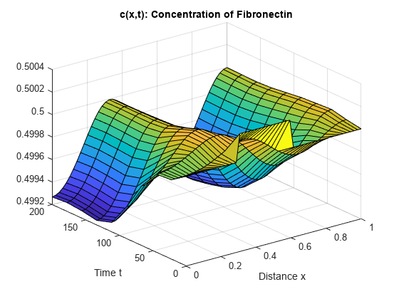
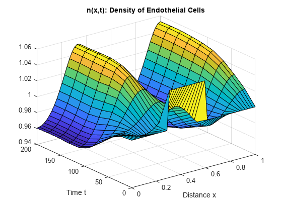
Create a surface plot of the solution components and plotted at the selected mesh points for and .
surf(x,t,c)
title('c(x,t): Concentration of Fibronectin')
xlabel('Distance x')
ylabel('Time t')
surf(x,t,n)
title('n(x,t): Density of Endothelial Cells')
xlabel('Distance x')
ylabel('Time t')
Now plot just the final distributions of the solutions at . These plots correspond to Figures 3 and 4 in [1].
plot(x,n(end,:))
title('Final distribution of n(x,t_f)')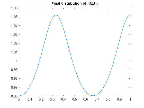
plot(x,c(end,:))
title('Final distribution of c(x,t_f)')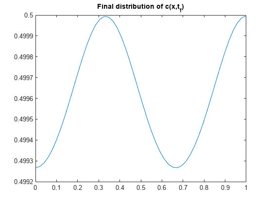
References
[1] Humphreys, M.E. and M.A.J. Chaplain. "A mathematical model of the first steps of tumour-related angiogenesis: Capillary sprout formation and secondary branching." IMA Journal of Mathematics Applied in Medicine & Biology, 13 (1996), pp. 73-98.
Local Functions
Listed here are the local helper functions that the PDE solver pdepe calls to calculate the solution. Alternatively, you can save these functions as their own files in a directory on the MATLAB path.
function [c,f,s] = angiopde(x,t,u,dudx) % Equation to solve
d = 1e-3;
a = 3.8;
S = 3;
r = 0.88;
N = 1;

c = [1; 1];
f = [d*dudx(1) - a*u(1)*dudx(2)
     dudx(2)];
s = [S*r*u(1)*(N - u(1));
     S*(u(1)/(u(1) + 1) - u(2))];
end
% ---------------------------------------------
function u0 = angioic(x) % Initial Conditions
u0 = [1; 0.5];
if x >= 0.3 && x <= 0.6
  u0(1) = 1.05 * u0(1);
  u0(2) = 1.0005 * u0(2);
end
end
% ---------------------------------------------
function [pl,ql,pr,qr] = angiobc(xl,ul,xr,ur,t) % Boundary Conditions
pl = [0; 0];
ql = [1; 1];
pr = pl;
qr = ql;
end
% ---------------------------------------------