dissect

Nested dissection permutation

Syntax

p = dissect(A)

p = dissect(A,Name,Value)

Description

p = dissect(A) returns a permutation vector computed using nested dissection of the sparsity structure of A.

p = dissect(A,Name,Value) specifies additional options using one or more name-value pair arguments. For example, dissect(A,'NumIterations',15) uses 15 refinement iterations in the nested dissection algorithm instead of 10.

Examples

Reorder Sparse Matrix Columns

Reorder a sparse matrix with several methods and compare the fill-in incurred by the LU decomposition of the reordered matrices.

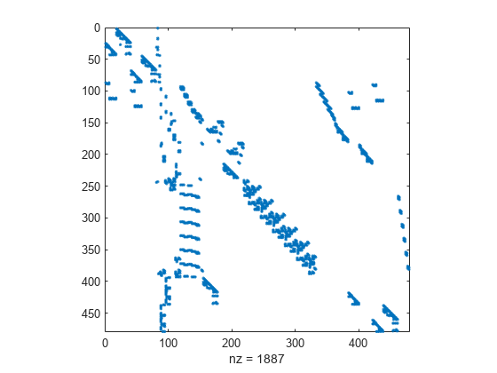
Load the west0479 matrix, which is a real-valued 479-by-479 sparse matrix with both real and complex pairs of conjugate eigenvalues. View the sparsity structure.

load west0479.mat
A = west0479;
spy(A)

Calculate several different permutations of the matrix columns, including the nested dissection ordering.

p1 = dissect(A);
p2 = amd(A);
p3 = symrcm(A);

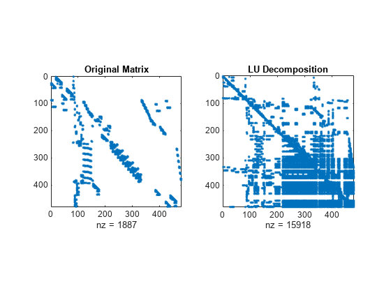
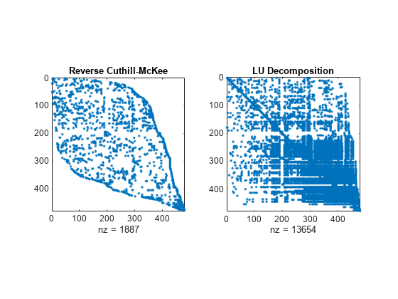
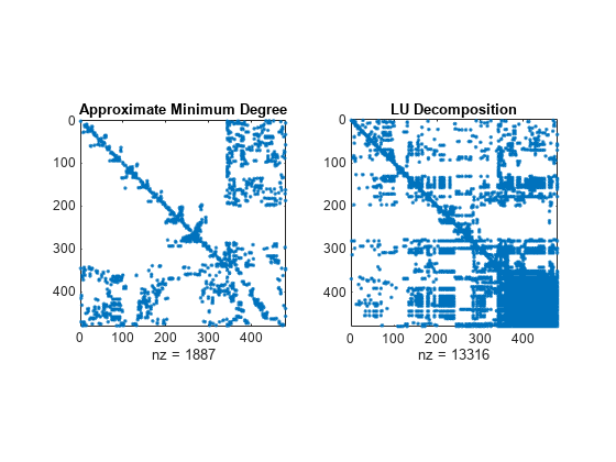
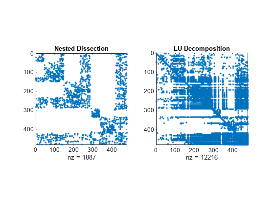
Compare the sparsity structures of the LU decomposition of A using the different ordering methods. The dissect function produces the reordering that incurs the least amount of fill-in.

subplot(1,2,1)
spy(A)
title('Original Matrix')
subplot(1,2,2)
spy(lu(A))
title('LU Decomposition')

figure
subplot(1,2,1)
spy(A(p3,p3))
title('Reverse Cuthill-McKee')
subplot(1,2,2)
spy(lu(A(p3,p3)))
title('LU Decomposition')

figure
subplot(1,2,1)
spy(A(p2,p2))
title('Approximate Minimum Degree')
subplot(1,2,2)
spy(lu(A(p2,p2)))
title('LU Decomposition')

figure
subplot(1,2,1)
spy(A(p1,p1))
title('Nested Dissection')
subplot(1,2,2)
spy(lu(A(p1,p1)))
title('LU Decomposition')

Filter Out Dense Columns

An arrowhead matrix is a sparse matrix that has a few dense columns. Use the 'MaxDegreeThreshold' name-value pair to filter the dense columns to the end of the reordered matrix.

Create an arrowhead sparse matrix and view the sparsity pattern.

A = speye(100) + diag(ones(1,99),1) + diag(ones(1,98),2);
A(1:5,:) = ones(5,100);
A = A + A';
spy(A)

Calculate the nested dissection ordering, and filter out the columns that have more than 10 nonzero elements.

p = dissect(A,'MaxDegreeThreshold',10);

View the sparsity pattern of the reordered matrix. dissect places the dense columns at the end of the reordered matrix.

spy(A(p,p))

Input Arguments

A — Input matrix

square matrix

Input matrix, specified as a square matrix. A can be either full or sparse. If A is nonsymmetric, then dissect symmetrizes it.

Data Types: single | double | int8 | int16 | int32 | int64 | uint8 | uint16 | uint32 | uint64 | logical
Complex Number Support: Yes

Name-Value Arguments

Specify optional pairs of arguments as Name1=Value1,...,NameN=ValueN, where Name is the argument name and Value is the corresponding value. Name-value arguments must appear after other arguments, but the order of the pairs does not matter.

Before R2021a, use commas to separate each name and value, and enclose Name in quotes.

Example: p = dissect(A,'NumIterations',15,'NumSeparators',2) uses 15 refinement iterations and 2 separators in the nested dissection algorithm.

VertexWeights — Vertex weights

vector

Vertex weights, specified as the comma-separated pair consisting of 'VertexWeights' and a vector. The vector of weights must have length equal to size(A,1) so that a weight is specified for each vertex. Use this option to specify how the graph vertices (matrix columns) are weighted, which affects how the algorithm computes the balance between partitions.

By default, the nested dissection algorithm weights all vertices equally.

Data Types: single | double | int8 | int16 | int32 | int64 | uint8 | uint16 | uint32 | uint64

NumSeparators — Number of separators

1 (default) | positive integer

Number of separators, specified as the comma-separated pair consisting of 'NumSeparators' and a positive integer. Use this option to specify how many partitions the graph is split into during each partitioning step. Increasing the number of separators in the nested dissection algorithm can result in a higher quality permutation at the cost of additional execution time.

Data Types: single | double | int8 | int16 | int32 | int64 | uint8 | uint16 | uint32 | uint64

NumIterations — Number of refinement iterations

10 (default) | positive integer

Number of refinement iterations, specified as the comma-separated pair consisting of 'NumIterations' and a positive integer. More refinement iterations can result in a higher quality permutation at the cost of increased execution time.

Data Types: single | double | int8 | int16 | int32 | int64 | uint8 | uint16 | uint32 | uint64

MaxImbalance — Threshold for partition imbalance

1.2 (default) | scalar

Threshold for partition imbalance, specified as the comma-separated pair consisting of 'MaxImbalance' and a scalar value that is an integer multiple of 0.001 greater than or equal to 1.001 and less than or equal to 1.999. Larger threshold values might reduce execution time by allowing the algorithm to accept a worse permutation.

Data Types: single | double

MaxDegreeThreshold — Threshold for vertex degree

0 (default) | nonnegative integer

Threshold for vertex degree, specified as the comma-separated pair consisting of 'MaxDegreeThreshold' and a nonnegative integer. The nested dissection algorithm ignores vertices with degree larger than threshold*(avg degree)/10 during ordering. dissect places vertices ignored in this way at the end of the permutation. This effectively places any vertices with degree greater than the threshold in the first, top-level separator. Filtering out highly connected vertices can sometimes improve the speed and accuracy of the ordering.

The default value of 0 means that all vertices are ordered.

Data Types: single | double | int8 | int16 | int32 | int64 | uint8 | uint16 | uint32 | uint64

Output Arguments

p — Permutation vector

vector

Permutation vector, returned as a vector. Use the permutation vector to reorder the columns of A using the indexing expression A(p,p). For example, the Cholesky factorization chol(A(p,p)) tends to be sparser than that of A.

Algorithms

The nested dissection ordering algorithm described in [1] is a multilevel graph partitioning algorithm that is used to produce fill-reducing orderings of sparse matrices. The input matrix is treated as the adjacency matrix of a graph. The algorithm coarsens the graph by collapsing vertices and edges, reorders the smaller graph, and then uses refinement steps to uncoarsen the small graph and produce a reordering of the original graph.

The name-value pairs for dissect enable you to control various stages of the algorithm:

• Coarsening

  In this phase, the algorithm creates successively smaller graphs from the original graph by collapsing together adjacent pairs of vertices. 'MaxDegreeThreshold' enables you to filter out highly connected graph vertices (which are dense columns in the matrix) by ordering them last.

• Partitioning

  After the graph is coarsened, the algorithm completely reorders the smaller graph. At each partitioning step, the algorithm attempts to partition the graph into equal parts: 'NumSeparators' specifies how many parts to partition the graph into, 'VertexWeights' optionally assigns weights to the vertices, and 'MaxImbalance' specifies the threshold for the difference in weight between the different partitions.

• Refinement

  After the smallest graph is reordered, the algorithm makes projections to enlarge the graph back to the original size by expanding the vertices that were previously combined. After each projection step, a refinement step is performed that moves vertices between partitions to improve the quality of the solution. 'NumIterations' controls how many refinement steps are used during this uncoarsening phase.

References

[1] Karypis, George and Vipin Kumar. "A Fast and High Quality Multilevel Scheme for Partitioning Irregular Graphs." SIAM Journal on Scientific Computing. Vol. 20, Number 1, 1999, pp. 359–392.

Extended Capabilities

Thread-Based Environment

Run code in the background using MATLAB® backgroundPool or accelerate code with Parallel Computing Toolbox™ ThreadPool.

This function fully supports thread-based environments. For more information, see Run MATLAB Functions in Thread-Based Environment.

Version History

Introduced in R2017b