mpcmove

Compute optimal control action and update controller states

Syntax

mv = mpcmove(MPCobj,xc,ym,r,v)

[mv,info] = mpcmove(MPCobj,xc,ym,r,v)

[___] = mpcmove(___,options)

Description

Use this command to simulate an MPC controller in closed-loop with a plant model. Call mpcmove repeatedly in a for loop to calculate the manipulated variable and update the controller states at each time step.

mv = mpcmove(MPCobj,xc,ym,r,v) returns the optimal move mv and updates the states xc of the controller MPCobj.

The manipulated variable mv at the current time is calculated given:

• the controller object, MPCobj,

• a pointer to the current estimated extended state, xc,

• the measured plant outputs, ym,

• the output references, r,

• and the measured disturbance input, v.

If ym, r or v is specified as [], or if it is missing as a last input argument, mpcmove uses the appropriate MPCobj.Model.Nominal value instead.

When using default state estimation, mpcmove also updates the controller state referenced by the handle object xc. Therefore, when using default state estimation, xc always points to the updated controller state. When using custom state estimation, you should update xc prior to each mpcmove call.

[mv,info] = mpcmove(MPCobj,xc,ym,r,v) returns additional information about the optimization problem solved to calculate mv.

[___] = mpcmove(___,options) overrides default constraints and weights in MPCobj with the values specified in Options, an mpcmoveopt object. Use Options to provide run-time adjustment of constraints and weights during the closed-loop simulation.

Examples

Simulate Closed-Loop Response Using mpcMove

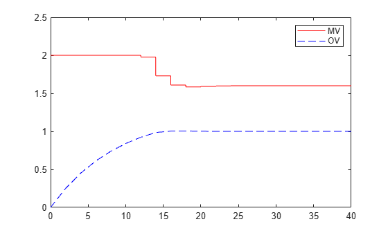
Perform closed-loop simulation of a plant with one MV and one measured OV.

Define a plant model and create a model predictive controller with MV constraints.

ts = 2;
Plant = ss(0.8,0.5,0.25,0,ts);
mpcobj = mpc(Plant);

-->The "PredictionHorizon" property is empty. Assuming default 10.
-->The "ControlHorizon" property is empty. Assuming default 2.
-->The "Weights.ManipulatedVariables" property is empty. Assuming default 0.00000.
-->The "Weights.ManipulatedVariablesRate" property is empty. Assuming default 0.10000.
-->The "Weights.OutputVariables" property is empty. Assuming default 1.00000.

mpcobj.MV(1).Min = -2;
mpcobj.MV(1).Max = 2;

Obtain an handle object pointing to the controller state.

xc = mpcstate(mpcobj)

-->Assuming output disturbance added to measured output channel #1 is integrated white noise.
-->The "Model.Noise" property is empty. Assuming white noise on each measured output.
MPCSTATE object with fields
          Plant: 0
    Disturbance: 0
          Noise: [1x0 double]
       LastMove: 0
     Covariance: [2x2 double]

The controller has one state for the internal plant model, one for the disturbance model, and one to hold the last value of the manipulated variable. All these three states are initialized to zero.

Set the reference signal. There is no measured disturbance.

r = 1;

Simulate the closed-loop response by calling mpcmove iteratively. In the simulation, assume that the simulated plant is identical to the predictive model. Therefore the plant state x in this case is identical to xc.Plant and the plant output is y = C*x + D*u = 0.25*x = 0.25*xc.Plant. Here, mpcmove updates the controller state referenced by xc (therefore including xc.Plant), and returns the manipulated variable in u(i), which is used just for plotting.

t = 0:ts:40;
N = length(t);
y = zeros(N,1); 
u = zeros(N,1); 
for i = 1:N
    y(i) = 0.25*xc.Plant;
    u(i) = mpcmove(mpcobj,xc,y(i),r);
end

Analyze the result.

[ts,us] = stairs(t,u);
plot(ts,us,'r-',t,y,'b--')
legend('MV','OV')

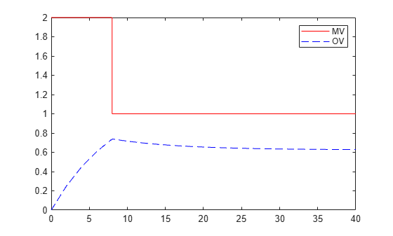
Modify the MV upper bound as the simulation proceeds using an mpcmoveopt object. Since the options argument overrides selected mpcobj properties, specify MV constraints again.

MPCopt = mpcmoveopt;
MPCopt.MVMin = -2;
MPCopt.MVMax = 2;

Simulate the closed-loop response and introduce the real-time upper limit change at eight seconds (the fifth iteration step).

xc = mpcstate(mpcobj);
y = zeros(N,1);
u = zeros(N,1);
for i = 1:N
    y(i) = 0.25*xc.Plant;
    if i == 5
    	MPCopt.MVMax = 1;
    end
    u(i) = mpcmove(mpcobj,xc,y(i),r,[],MPCopt);
end

Analyze the results.

[ts,us] = stairs(t,u);
plot(ts,us,'r-',t,y,'b--')
legend('MV','OV')

Evaluate Scenario at Specific Time Instant

Define a plant model.

ts = 2;
Plant = ss(0.8,0.5,0.25,0,ts);

Create a model predictive controller with constraints on both the manipulated variable and the rate of change of the manipulated variable. The prediction horizon is 10 intervals, and the control horizon is blocked.

MPCobj = mpc(Plant,ts,10,[2 3 5]);

-->The "Weights.ManipulatedVariables" property is empty. Assuming default 0.00000.
-->The "Weights.ManipulatedVariablesRate" property is empty. Assuming default 0.10000.
-->The "Weights.OutputVariables" property is empty. Assuming default 1.00000.

MPCobj.MV(1).Min = -2;
MPCobj.MV(1).Max = 2;
MPCobj.MV(1).RateMin = -1;
MPCobj.MV(1).RateMax = 1;

Initialize (and return an handle to) the controller internal state for simulation.

xc = mpcstate(MPCobj);

-->Assuming output disturbance added to measured output channel #1 is integrated white noise.
-->The "Model.Noise" property is empty. Assuming white noise on each measured output.

xc.Plant = 2.8;
xc.LastMove = 0.85;

Compute the optimal control move at the current time.

y = 0.25*xc.Plant;
r = 1;
[u,Info] = mpcmove(MPCobj,xc,y,r);

Analyze the predicted optimal sequences.

[ts,us] = stairs(Info.Topt,Info.Uopt);
plot(ts,us,'r-',Info.Topt,Info.Yopt,'b--')
legend('MV','OV')

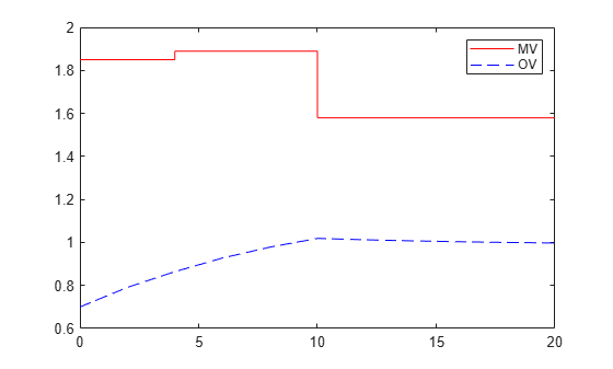
plot ignores Info.Uopt(end) as it is NaN.

Examine the optimal cost.

Info.Cost

ans = 0.0793

Input Arguments

MPCobj — Model predictive controller

MPC controller object

Model predictive controller, specified as an MPC controller object. To create an MPC controller, use mpc.

xc — Handle object pointing to current controller state

mpcstate handle object

Handle object pointing to current controller state, specified as an mpcstate object.

Note

Since xc is an handle object, if you copy it to a new variable, the new variable still points to the current state of the same mpc object. If this state changes, this is reflected in both xc and its copy. To preserve the original state for later use, you can save xc to a MAT-file. During simulation, mpcmove also updates xc when a new control move is calculated. For more information about handle objects, see Handle Object Behavior.

Before you begin a simulation with mpcmove, initialize the controller, and return an handle to its state using xc = mpcstate(MPCobj). Then, modify the default properties of xc as appropriate. mpcmove modifies the controller state. The handle object xc always reflect the current (updated) state of the controller.

If you are using default state estimation, mpcmove expects xc to represent xc[n|n-1]. The mpcmove command updates the state values in the previous control interval with that information. Therefore, you should not programmatically update xc at all. The default state estimator employs a steady-state Kalman filter.

If you are using custom state estimation, mpcmove expects xc to represent xc[n|n]. Therefore, prior to each mpcmove command, you must set xc.Plant, xc.Disturbance, and xc.Noise to the best estimates of these states (using the latest measurements) at the current control interval.

ym — Current measured output values

column vector of length N_ym

Current measured output values at time k, specified as a column vector of length N_ym, where N_ym is the number of measured outputs.

If you are using custom state estimation, set ym = [].

r — Plant output reference values

p-by-N_y array

Plant output reference values, specified as a p-by-N_y array, where p is the prediction horizon of MPCobj and N_y is the number of outputs. Row r(i,:) defines the reference values at step i of the prediction horizon.

r must contain at least one row. If r contains fewer than p rows, mpcmove duplicates the last row to fill the p-by-N_y array. If you supply exactly one row, therefore, a constant reference applies for the entire prediction horizon.

To implement reference previewing, which can improve tracking when a reference varies in a predictable manner, r must contain the anticipated variations, ideally for p steps.

v — Current and anticipated measured disturbances

(p+1)-by-N_md array

Current and anticipated measured disturbances, specified as a (p+1)-by-N_md array, where p is the prediction horizon of MPCobj and N_md is the number of measured disturbances. The first row of v specifies the current measured disturbance values. Row v(i+1,:) defines the anticipated disturbance values at step i of the prediction horizon.

Modeling of measured disturbances provides feedforward control action. If your plant model does not include measured disturbances, use v = [].

If your model includes measured disturbances, v must contain at least one row. If v contains fewer than p+1 rows, mpcmove duplicates the last row to fill the (p+1)-by-N_md array. If you supply exactly one row, a constant measured disturbance applies for the entire prediction horizon.

To implement disturbance previewing, which can improve tracking when a disturbance varies in a predictable manner, v must contain the anticipated variations, ideally for p steps.

options — Run-time options

mpcmoveopt object

Run-time options, specified as an mpcmoveopt object. Use options to override selected properties of MPCobj during simulation. These options apply to the current mpcmove time instant only. Using options yields the same result as redefining or modifying MPCobj before each call to mpcmove, but involves considerably less overhead. Using options is equivalent to using an MPC Controller Simulink^® block in combination with optional input signals that modify controller settings, such as MV and OV constraints.

Output Arguments

mv — Optimal manipulated variable moves

column vector

Optimal manipulated variable moves, returned as a column vector of length N_mv, where N_mv is the number of manipulated variables.

If the controller detects an infeasible optimization problem or encounters numerical difficulties in solving an ill-conditioned optimization problem, mv remains at its most recent successful solution, xc.LastMove.

Otherwise, if the optimization problem is feasible and the solver reaches the specified maximum number of iterations without finding an optimal solution, mv:

• Remains at its most recent successful solution if the Optimizer.UseSuboptimalSolution property of the controller is false.

• Is the suboptimal solution reached after the final iteration if the Optimizer.UseSuboptimalSolution property of the controller is true. For more information, see Suboptimal QP Solution.

info — Solution details

structure

Solution details, returned as a structure with the following fields.

Uopt — Optimal manipulated variable sequence

(p+1)-by-N_mv array

Predicted optimal manipulated variable adjustments (moves), returned as a (p+1)-by-N_mv array, where p is the prediction horizon and N_mv is the number of manipulated variables.

Uopt(i,:) contains the calculated optimal values at time k+i-1, for i = 1,...,p, where k is the current time. The first row of Info.Uopt contains the same manipulated variable values as output argument mv. Since the controller does not calculate optimal control moves at time k+p, Uopt(p+1,:) is equal to Uopt(p,:).

Yopt — Optimal output variable sequence

(p+1)-by-N_y array

Optimal output variable sequence, returned as a (p+1)-by-N_y array, where p is the prediction horizon and N_y is the number of outputs.

The first row of Info.Yopt contains the calculated outputs at time k based on the estimated states and measured disturbances; it is not the measured output at time k. Yopt(i,:) contains the predicted output values at time k+i-1, for i = 1,...,p+1.

Yopt(i,:) contains the calculated output values at time k+i-1, for i = 2,...,p+1, where k is the current time. Yopt(1,:) is computed based on the estimated states and measured disturbances.

Xopt — Optimal prediction model state sequence

(p+1)-by-N_x array

Optimal prediction model state sequence, returned as a (p+1)-by-N_x array, where p is the prediction horizon and N_x is the number of states in the plant and unmeasured disturbance models (states from noise models are not included).

Xopt(i,:) contains the calculated state values at time k+i-1, for i = 2,...,p+1, where k is the current time. Xopt(1,:) is the same as the current states state values.

Topt — Time intervals

column vector of length p+1

Time intervals, returned as a column vector of length p+1. Topt(1) = 0, representing the current time. Subsequent time steps Topt(i) are given by Ts*(i-1), where Ts = MPCobj.Ts is the controller sample time.

Use Topt when plotting the Uopt, Xopt, or Yopt sequences.

Slack — Slack variable

nonnegative scalar

Slack variable, ε, used in constraint softening, returned as 0 or a positive scalar value.

• ε = 0 — All constraints were satisfied for the entire prediction horizon.

• ε > 0 — At least one soft constraint is violated. When more than one constraint is violated, ε represents the worst-case soft constraint violation (scaled by your ECR values for each constraint).

See Optimization Problem for more information.

Iterations — Number of solver iterations

positive integer | 0 | -1 | -2

Number of solver iterations, returned as one of the following:

• Positive integer — Number of iterations needed to solve the optimization problem that determines the optimal sequences.

• 0 — Optimization problem could not be solved in the specified maximum number of iterations.

• –1 — Optimization problem was infeasible. An optimization problem is infeasible if no solution can satisfy all the hard constraints.

• –2 — Numerical error occurred when solving the optimization problem.

QPCode — Optimization solution status

'feasible' | 'infeasible' | 'unrealiable'

Optimization solution status, returned as one of the following:

• 'feasible' — Optimal solution was obtained (Iterations > 0)

• 'infeasible' — Solver detected a problem with no feasible solution (Iterations = –1) or a numerical error occurred (Iterations = –2)

• 'unreliable' — Solver failed to converge (Iterations = 0). In this case, if MPCobj.Optimizer.UseSuboptimalSolution is false, u freezes at the most recent successful solution. Otherwise, it uses the suboptimal solution found during the last solver iteration.

Cost — Objective function cost

nonnegative scalar

Objective function cost, returned as a nonnegative scalar value. The cost quantifies the degree to which the controller has achieved its objectives. For more information, see Optimization Problem.

The cost value is only meaningful when QPCode = 'feasible', or when QPCode = 'feasible' and MPCobj.Optimizer.UseSuboptimalSolution is true.

Tips

• mpcmove updates xc, even though it is an input argument.

• If ym, r or v is specified as [], or if it is missing as a last input argument, mpcmove uses the appropriate MPCobj.Model.Nominal value instead.

• To view the predicted optimal behavior for the entire prediction horizon, plot the appropriate sequences provided in Info.

• To determine the optimization status, check Info.Iterations and Info.QPCode.

Alternatives

• Use sim for plant mismatch and noise simulation when not using run-time constraints or weight changes.

• Use the MPC Designer app to interactively design and simulate model predictive controllers.

• Use the MPC Controller block in Simulink and for code generation.

• Use mpcmoveCodeGeneration to simulate an MPC controller prior to code generation.

Version History

Introduced before R2006a