Model Continuous-Time Low-Pass Delta-Sigma Modulator with Different Levels of Abstraction

Since R2025a

This example uses:

This example shows how to synthesize, model and simulate a $3^{rd}$ -order continuous-time (CT) low pass Delta-Sigma Modulator (LP-DSM), by using various levels of abstraction, starting from ideal/system-level model using Mixed-Signal Blockset's DSM block to a schematic model based on Simscape blocks.

A step-by-step procedure is described to synthesize the architecture, set main simulation parameter, select the model view (abstraction level), simulate the model and get main performance metrics.

Design Flow

The first step to design any Delta Sigma Modulator (DSM) is to obtain the best Noise Transfer Function (NTF) which maximizes the performance of a given modulator topology of a certain order( $3^{rd}$ -order in this case). The NTF is usually expressed as [1][2]:

$N T F (z) = \frac{1}{1 + L_{1} (z)}$

where $L_{1} (z)$ denotes the transfer function of the feedback filter of a discrete-time (DT) Delta Sigma Modulator, and can be easily obtained by using Richard Schrier's Delta-Sigma Toolbox [3] by properly setting main system parameters as follows:

L = 3;                              % Modulator order (fixed value for this example)
OSR = 64;                           % Oversampling ratio
opt = 0;                            % A flag used to request optimized NTF zeros [0, 3]

ntf = synthesizeNTF(L, OSR, opt);   % Synthesize the NTF [3]
L1_z = 1/ntf-1;                     % Definition of L1(z) as a function of NTF

(If you modify OSR, make sure to set appropriate values for the rest of parameters inside the Simulink model.)

Once the NTF of the DT DSM has been obtained, the impulse-invariant transformation (IIT) is applied to obtain the loop-filter coefficients of the equivalent Continuous-Time (CT) DSM. For instance, in the case of the $3^{rd}$ -order CT DSM in this example, the feedback filter is given by:

$L_{1} (s) = \frac{k_{1}}{s} + \frac{k_{2}}{s ²} + \frac{k_{3}}{s ³}$

where $k_{i}$ are the loop-filter coefficients [1].

The proposed methodology considers the impulse response for each node in the CT system, and its transformation into the discrete domain, where the equations are solved:

$[x_{1} x_{2} x_{3}] [k_{1} k_{2} k_{3}]^{'} = l$

where $x_{i}$ represent the impulse response of each node in the model, and $l$ stands for the impulse response of $L_{1} (z)$ .

l = impulse(L1_z, 10);                        % impulse response of the discrete model (10 samples)
x1 = impulse(c2d(tf(1, [1 0]), 1), 10);       % impulse response of term 1/s (10 samples)
x2 = impulse(c2d(tf(1, [1 0 0]), 1), 10);     % impulse response of term 1/s² (10 samples)
x3 = impulse(c2d(tf(1, [1 0 0 0]), 1), 10);   % impulse response of term 1/s³ (10 samples)
K = [x1 x2 x3]\l;                             % loop-filter coefficients for the CT model

Now that the coefficients have been obtained, the $3^{rd}$ -order modulator can be simulated for different abstraction levels. Starting with an ideal system description represented by DSM block shipped in Mixed-Signal Blockset, followed by a choice from available Simscape models that consider integrators blocks with following building blocks:

Op-Amp
Band-Limited Op-Amp
Fully Differential Op-Amp.

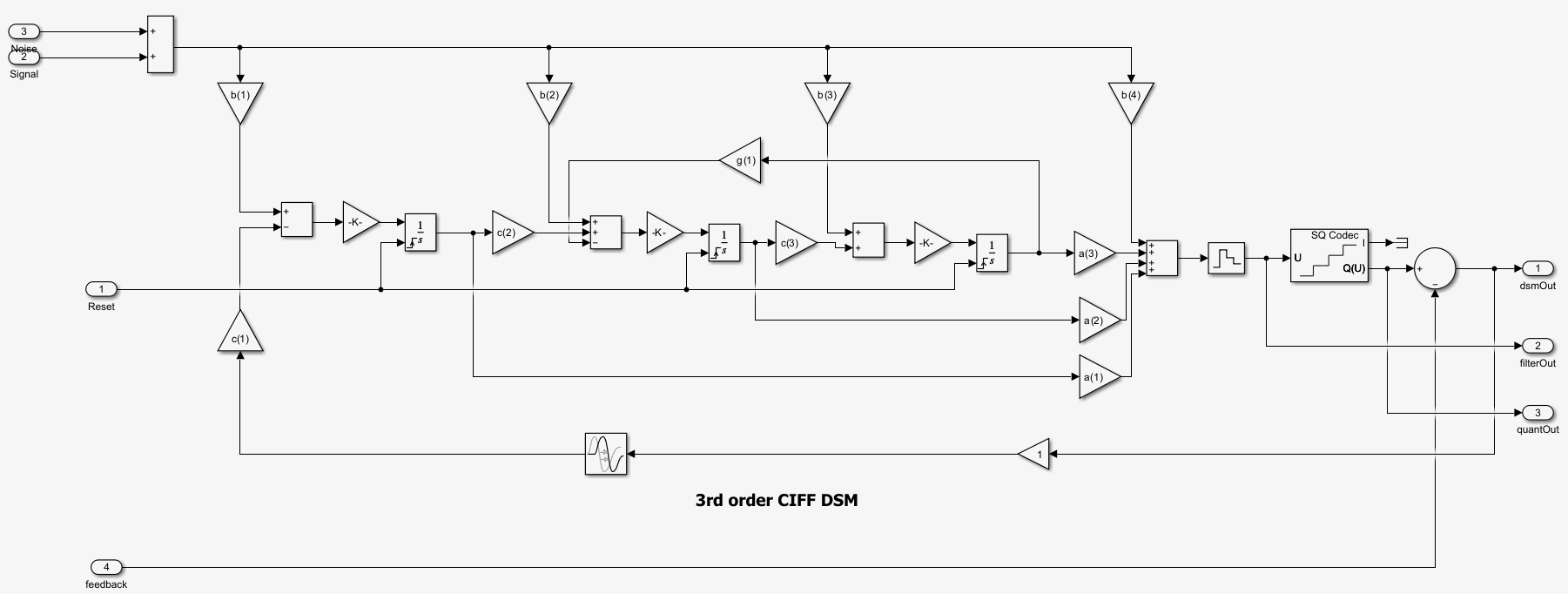
Continuous-Time Delta Sigma Modulator Design

Here is the Simulink representation of a 3rd-order Continuous-Time Delta Sigma Modulator as modeled in Mixed-Signal Blockset for cascade of integrators with feed-forward (CIFF) architecture.

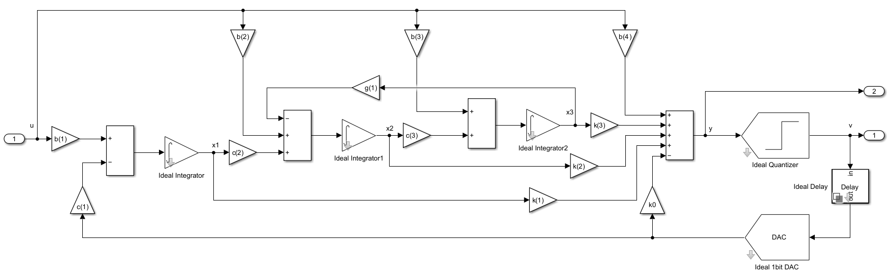
ELD implementation

Below is the simulink representation of CT-DSM with excess loop delay (ELD) modeled in the system.

Op-Amp

Screenshot shown below includes Simscape representation of an operational amplifier used to create a CT-DSM system with CIFF archiecture as above.

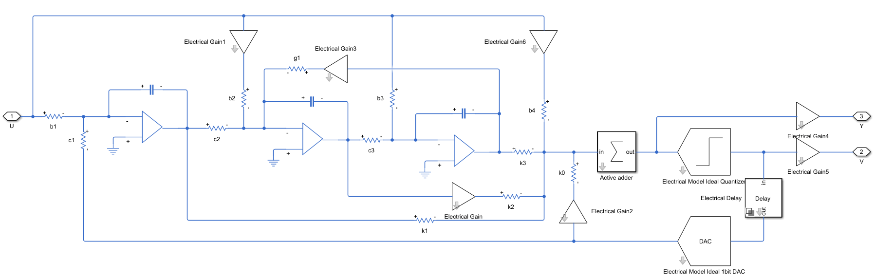
This design option allows user to map system-level loop-filter coefficients (ai, bi, ci...) into the corresponding circuit-level parameters by considering an active-RC circuit realization using opamps, resistors and capacitors. This enables the designer to see the effect of finite dc gain of amplifiers (Op-Amp). it is a static error which causes an increase of the in-band noise power and harmonic distortion, by reducing the Signal-to-Noise and Distortion (SNDR) ratio and hence, the effective number of bits (ENOB).

The image below further modifies the system shown above to include band-limited operation amplifier modeled using Simscape.

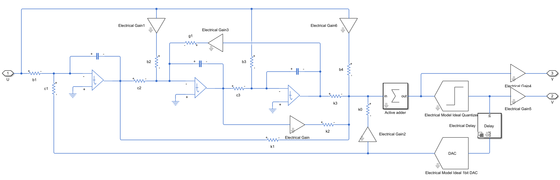
This implementation can be used to observe the effect of nonideal dynamics caused by band-limited Op-Amp, and more especifically the impact of finite Gain-BandWidth (GBW), which may also cause an increase of the noise floor. Although this effect is less critical in CT DSMs as compared to Switched-Capacitor (SC) counterparts, it must be taken into account when designing high-performance data converters.

All the models above consider a single-ended representation of the system. A more realistic circuit implementation consists of a fully-differential circuit.

As shown below a fully differential operation amplifier has been implemented using Simscape to create a CT-DSM system:

This is the most common way to implement high-performance DSMs in practice. This design option removes, among others, the effect of offset and even-order harmonics [1][2].

model = 0;     % model selection
open_system('ord_3rd_CIFF_CT_LP_all_models.slx');

The main parameters considered in this exampled are listed below:

Sampling frequency (fs) = 128 kHz

Bandwidth (Bw) = 1e3 kHz

Input signal amplitude (A) = 0.5 V

Input signal frequency (fin) = 990 kHz

Number of points for the FFT (N) = $2^{14}$

The following code recalculates loop-filter coefficients in order to consider the effect of ELD. This feature returns appropriate results only for model option of "Simulink: ELD implementation". It is recommended to set eld=0 if user simulates any other of the available models.

eld = 0;                 % excess loop delay (typical values: eld=1 | eld=1/2)

ELD = [1 eld eld^2/2; 0 1 eld; 0 0 1; eld eld^2/2 eld^3/6];
Kc = ELD*K;
if model == 1
    K = Kc(1:end-1);     % recalculated loop-filter coefficients
end
K0 = Kc(end);            % loop-filter coefficient of the additional path

The topology can be simulated at a lower abstraction level (electrical-level description), by including different behavioral models for the amplifiers used to build the integrators in the loop. These electrical models consider either single-ended or fully-differential implementations, with several circuit nonidealities. Each model uses a different amplifier representation from Simscape : Op-amp, band-limited op-amp or fully differential op-amp.

Evaluate DSM Performance

Here is the testbench setup for the DSM that's used to evaluate its performance:

Once all modulator parameters have been set, you can proceed to simulate the model for the selected abstraction level.

out = sim('ord_3rd_CIFF_CT_LP_all_models.slx');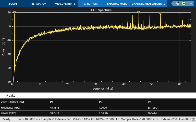

The scope of the spectrum analyzer depicts the FFT spectrum of the output signal. It illustrates how the quantization noise is shaped so that it is pushed out of the band of interest.

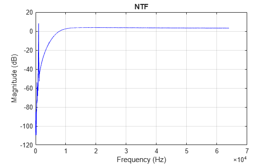
The simulation also returns to the workspace, values of the input signal (U), the output of the modulator (V) and the signal at the input of the quantizer (Y). It is feasible to plot the NTF by processing these values through a script as given below:

N = 2^14;                                                   % Points for FFT
fs = 128e3;                                                 % sampling frequency
f = (1:N/2)*(fs/N);                                         % frequency array
w = hanning(N);                                             % window to apply over the processed signals
specV = 20*log10(2*abs(fft(out.v.*w))/sum(w));              % FFT spectrum of V
specVY = 20*log10(2*abs(fft((out.v-out.y).*w))/sum(w));     % FFT spectrum of V-Y
specNTF = specV-specVY;                                     % shape of the NTF

figure('Name','NTF');
plot(f, specNTF(1:N/2), 'b');
title('NTF'); xlabel('Frequency (Hz)'); ylabel('Magnitude (dB)');
grid on;

Figure NTF contains an axes object. The axes object with title NTF, xlabel Frequency (Hz), ylabel Magnitude (dB) contains an object of type line.

Eventually, the output of the DSM feeds an 'FIR decimator' which filters the out-of-band noise and decimates the bitstream. Additionally, one can also use 'ADC AC Measurement' block from Mixed-Signal Blockset in order to evaluate figures of merit, such as signal-to-noise ratio (SNR) and effective number of bits (ENOB):

FoM = table(adc_ac_out.SNR, adc_ac_out.ENOB, 'VariableNames',{'SNR', 'ENOB'});
disp(FoM);

     SNR      ENOB 
    ______    _____

    73.035    11.84

Comparing the results obtained from the 5 different representation of DSM we can see a pattern of expected behavior. For all cases we see similar SNR and ENOB performances.

Conclusion

This example shows how to model, simulate and obtain main performance metrics of an unscaled $3^{rd}$ -order Delta-Sigma Modulator (DSM) . Different abstraction levels (from ideal/system-level model to electrical models) taking circuit nonidealities into account can be considered in the simulation. Other DSM topologies can be simulated by using the architecture options available in the DSM block shipped in Mixed-Signal Blockset.

References

[3] Richard Schreier (2022). Delta Sigma Toolbox (https://www.mathworks.com/matlabcentral/fileexchange/19-delta-sigma-toolbox), MATLAB Central File Exchange. Retrieved June 14, 2022.

References

[1] Shanthi Pavan; Richard Schreier; Gabor C. Temes, Understanding Delta-Sigma Data Converters, Wiley-IEEE Press, second edition, copyright 2017.
[2] Jose M. de la Rosa, Sigma-Delta Converters: Practical Design Guide, Wiley-IEEE Press, second edition, copyright 2018.