boustrophedonOptions

Options for boustrophedon polygon decomposition algorithm

Since R2025a

Description

The boustrophedonOptions object defines the behavior of polygon decomposition using the boustrophedon algorithm and enables you to generate a connectivity graph of polygon cells post-decomposition. Specify this object to the polygonDecomposition function to perform decomposition using the boustrophedon decomposition algorithm with the specified options [1].

Creation

Syntax

options = boustrophedonOptions

options = boustrophedonOptions(PropertyName=Value)

Description

options = boustrophedonOptions generates a polygon decomposition options object with default properties. Specify this object to the polygonDecomposition function to perform decomposition using the boustrophedon decomposition algorithm with the specified options.

options = boustrophedonOptions(PropertyName=Value) sets one or more properties for options using name-value arguments.

Properties

ReturnConnectivity — Decomposition generates and returns connectivity graph

true or 1 (default) | false or 0

Decomposition generates and returns a connectivity graph, specified as a logical true (1) or false (0):

• false — Do not generate a connectivity graph.

  Note

  When ReturnConnectivity is false, the ReconnectionMethod, ConnectedCostFcn, DisconnectedCostFcn, and UserData properties have no effect.

• true — Generate a navGraph object representing the connectivity between cells in the polygon decomposition output, and return the navGraph in the solnInfo argument of the polygonDecomposition function.

ReconnectionMethod — Method to use to connect unconnected polygon clusters

"none" (default) | "nearest" | "all"

Method to connect groups of polygon clusters, specified as one of these options:

• "none" — Do not connect unconnected polygon clusters.

• "nearest" — Connect polygon clusters by the minimum distance edge between the polygon clusters.

• "all" — Connect every cell within a connected polygon cluster to every cell outside that cluster.

• Note

  The "nearest" and "all" options use the DisconnectedCostFcn property to determine the distance and the resulting edge costs between polygon clusters.

For more information about how ReconnectionMethod works, see Specify Options for Polygon Decomposition.

ConnectedCostFcn — Function for computing distance between sets of neighboring polygons

"boustrophedonOptions.defaultConnectedCostFcn" (default) | function name

Function for computing distance and edge costs between sets of neighboring polygons, specified as a function name. Neighboring polygons are polygons that share edges with each other.

Using the default "boustrophedonOptions.defaultConnectedCostFcn" function, the cost of connecting adjacent polygons is 0.

Cost functions must be of the form:

function cost = costFcn(polySet,i,J,userData)
    arguments (Inputs)
        polySet {mustBeA(polySet,{'polyshape','nav.decomp.internal.polyshapeMgr'})}
        i (1,1) {mustBeInteger,mustBePositive}
        J (:,1) {mustBeInteger,mustBePositive}
        userData (1,1) struct %#ok<INUSA>
    end
    arguments (Outputs)
        cost (:,1)
    end
    ...
end

For an example of how to specify ConnectedCostFcn, see Define Custom Connected Cost Function and User Data.

Data Types: char | string

DisconnectedCostFcn — Function for computing distance between nonneighboring polygons

"boustrophedonOptions.defaultDisconnectedCostFcn" (default) | function name

Function for computing distance cost between sets of nonneighboring polygons, specified as a function name. Nonneighboring polygons are polygons that do not share an edge with each other.

Using the default "boustrophedonOptions.defaultDisconnectedCostFcn" function, the cost of connecting nonneighboring polygons is the distance between polygon centroids.

Cost functions must be of the form:

function cost = costFcn(polySet,i,J,userData)
    arguments (Inputs)
        polySet {mustBeA(polySet,{'polyshape','nav.decomp.internal.polyshapeMgr'})}
        i (1,1) {mustBeInteger,mustBePositive}
        J (:,1) {mustBeInteger,mustBePositive}
        userData (1,1) struct %#ok<INUSA>
    end
    arguments (Outputs)
        cost (:,1)
    end
    ...
end

For an example of how to specify DisconnectedCostFcn, see Define Disconnected Cost Function.

UserData — Data for cost functions

struct([]) (default) | structure

Data for cost functions, specified as a structure. Store any data that you need for the cost functions as fields of this structure.

For an example of how to specify UserData, see Define Custom Connected Cost Function and User Data.

Examples

Specify Options for Polygon Decomposition

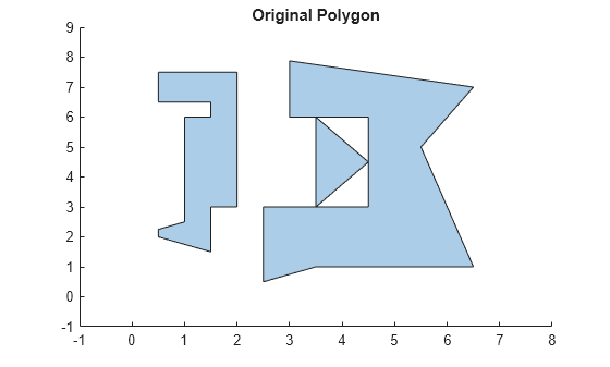
Load a polyshape and plot it.

load("exampleComplexPolyshape.mat","p")
plot(p)
title("Original Polygon")

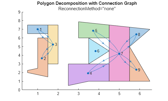
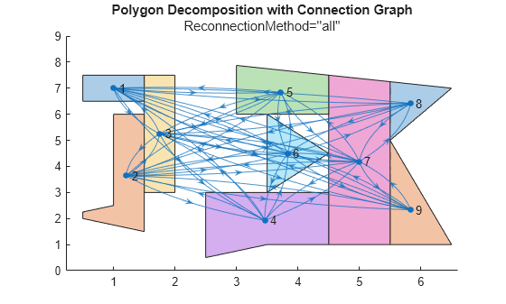
Decompose the polygon using each reconnection method.

bOpts1 = boustrophedonOptions(ReconnectionMethod="nearest");
[polySet1,info1] = polygonDecomposition(p,bOpts1);
bOpts2 = boustrophedonOptions(ReconnectionMethod="none");
[polySet2,info2] = polygonDecomposition(p,bOpts2);
bOpts3 = boustrophedonOptions(ReconnectionMethod="all");
[polySet3,info3] = polygonDecomposition(p,bOpts3);

Show the polygon decomposition with a connectivity graph overlay for each reconnection method.

plot(polySet1)
hold on
exampleHelperShowGraphConnectionsOnPolyset(polySet1,info1.Connectivity,0.5);
title("Polygon Decomposition with Connection Graph");
subtitle("ReconnectionMethod=''nearest''")
hold off

plot(polySet2)
hold on
exampleHelperShowGraphConnectionsOnPolyset(polySet2,info2.Connectivity,0.5);
title("Polygon Decomposition with Connection Graph");
subtitle("ReconnectionMethod=''none''");
hold off

plot(polySet3)
hold on
exampleHelperShowGraphConnectionsOnPolyset(polySet3,info3.Connectivity,0.5);
title("Polygon Decomposition with Connection Graph");
subtitle("ReconnectionMethod=''all''");
hold off

This is the helper function for plotting the polygon decomposition and overlaying the connectivity graph.

function gHandle = exampleHelperShowGraphConnectionsOnPolyset(polySet,connectionGraph,lineWidth)

    % Get the current axes
    ax = gca;
    ax.ColorOrderIndex = 1; % Reset the color order index

    % Overlay the connectivity graph
    gHandle = show(connectionGraph);
    gHandle.EdgeAlpha = 0.75;
    gHandle.LineWidth = lineWidth; % Set the line width for the graph edges

    % Calculate and plot the centroids
    [cx,cy] = centroid(polySet);

    % Set the xy-positions of the connectivity graph to the centroids of 
    % the polygons
    gHandle.XData = cx';
    gHandle.YData = cy';
end

Define Custom Connected Cost Function and User Data

Load a rectangular polygon with multiple holes as a polyshape object.

load("exampleRectangleWithHolesPolyshape.mat","p")

Define a connected cost function that uses terrain data and assigns costs to edges based on the magnitude of the slope change.

function cost = terrainConnectedCostFcn(polySet,i,J,userData)
    arguments
        polySet {mustBeA(polySet,{'polyshape','nav.decomp.internal.polyshapeMgr'})}
        i (1,1) {mustBeInteger,mustBePositive}
        J (:,1) {mustBeInteger,mustBePositive}
        userData (1,1) struct
    end

    % Extract dx, dy, and the coordinate bounds from userData
    dx = userData.XSlope;
    dy = userData.YSlope;
    xBounds = userData.XBounds;
    yBounds = userData.YBounds;

    % Calculate the slope magnitude
    slope_magnitude = sqrt(dx.^2 + dy.^2);

    % Define the coordinates for the slope map based on the provided bounds
    x = linspace(xBounds(1),xBounds(2),size(slope_magnitude,1));
    y = linspace(yBounds(1),yBounds(2),size(slope_magnitude,2));

    % Initialize the cost array
    cost = zeros(size(J));

    % Calculate the average slope for the starting polyshape
    avgSlope_i = calculateAverageSlope(polySet(i),slope_magnitude,x,y);

    for idx = 1:numel(J)
        % Calculate the average slope for each target polyshape
        avgSlope_j = calculateAverageSlope(polySet(J(idx)),slope_magnitude,x,y);

        % Define a cost function that includes the average slope difference
        % For example, prioritize smaller slope differences
        cost(idx) = abs(avgSlope_i-avgSlope_j);
    end
end

function avgSlope = calculateAverageSlope(poly,slope_magnitude,x,y)
    % Find the bounding box of the polyshape
    [x_lim,y_lim] = boundingbox(poly);

    % Determine the indices in the slope map that correspond to this
    % polyshape
    x_indices = find(x >= x_lim(1) & x <= x_lim(2));
    y_indices = find(y >= y_lim(1) & y <= y_lim(2));

    % Extract the relevant portion of the slope map
    slopesInPoly = slope_magnitude(y_indices,x_indices);

    % Compute the average slope for the polyshape
    avgSlope = mean(slopesInPoly(:));
end

Define custom data for the cost functions to use. Create an L-membrane to represent terrain, and calculate the slope at each point.

Z = membrane(1,3);
[dx,dy] = gradient(Z);

Store the slope and bounds data in a structure.

terrainData.XSlope = dx;
terrainData.YSlope = dy;
terrainData.XBounds = [1 8];
terrainData.YBounds = [1 8];

Create a boustrophedon options object, and specify the custom connected cost function and terrain data.

bOpts = boustrophedonOptions(ConnectedCostFcn="terrainConnectedCostFcn",UserData=terrainData);

Decompose the polygon and plot the set of resulting polygons.

[polySet,info] = polygonDecomposition(p,bOpts);
plot(polySet)
axis equal
hold on

Overlay the connectivity graph, and highlight the edges to show the edge costs between the decomposed polygons. Note that the peak of the L-membrane is around polygons 8, 11, and 13, so edges connecting these polygons to polygons in the top-left have a higher edge cost.

gHandle = exampleHelperShowGraphConnectionsOnPolyset(polySet,info.Connectivity,2);
exampleHelperVisualizeConnectionGraphWeights(info.Connectivity,gHandle);
title("Connection Graph with Cost Visualized")
customLinkInfo = info.Connectivity.Links

customLinkInfo=44×2 table
    EndStates     Weight 
    _________    ________

     1    2      0.090406
     1    3      0.026001
     1    4       0.27418
     2    1      0.090406
     2    5             0
     3    1      0.026001
     3    5       0.11641
     3    6       0.29335
     4    1       0.27418
     4    6       0.04517
     5    2             0
     5    3       0.11641
     5    7      0.062287
     5    8        0.4142
     6    3       0.29335
     6    4       0.04517
      ⋮

hold off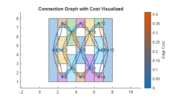

Define Disconnected Cost Function

Load a complex polyshape.

load exampleComplexPolyshape.mat

Define a custom disconnected cost function that prioritizes reconnecting the disconnected polygons using the longest edge possible.

function cost = longEdgeDisconnectedCostFcn(polySet,i,J,userData)
    arguments
        polySet {mustBeA(polySet,{'polyshape','nav.decomp.internal.polyshapeMgr'})}
        i (1,1) {mustBeInteger,mustBePositive}
        J (:,1) {mustBeInteger,mustBePositive}
        userData (1,1) struct %#ok<INUSA>
    end
    c1 = [0 0];
    c2 = zeros(numel(J),2);

    % Calculate the centroid of the current polygon
    [c1(1),c1(2)] = polySet(i).centroid;

    % Get the centroids of possible polygons connections
    for i = 1:numel(J)
        [c2(i,1),c2(i,2)] = polySet(J(i)).centroid;
    end

    % Calculate the centroid distances between the current polygon and
    % other polygons
    distances = vecnorm(c2-c1,2,2);

    % Calculate the inverse distance cost. Add a small number to avoid
    % division by zero
    cost = 1./(distances + 1e-6);
end

Create a boustrophedon polygon decomposition options object, and specify the disconnected cost function.

bOpts = boustrophedonOptions(DisconnectedCostFcn="longEdgeDisconnectedCostFcn", ...
    ReconnectionMethod="nearest");

Decompose the polygon and visualize the graph connection.

[polySet,info] = polygonDecomposition(p,bOpts);
plot(polySet)
hold on
gHandle = exampleHelperShowGraphConnectionsOnPolyset(polySet,info.Connectivity,0.5);
info.Connectivity.Links

ans=16×2 table
    EndStates    Weight 
    _________    _______

     1    3            0
     1    6      0.26465
     1    9      0.14884
     2    3            0
     3    1            0
     3    2            0
     4    7            0
     5    7            0
     6    1      0.26465
     7    4            0
     7    5            0
     7    8            0
     7    9            0
     8    7            0
     9    1      0.14884
     9    7            0

c = colororder;

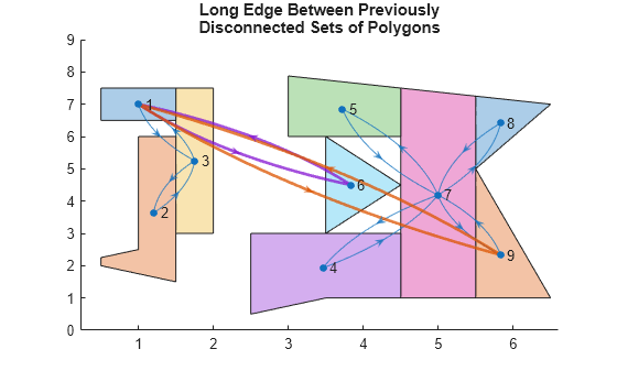
Highlight the edges between the previously disconnected sets of polygons. Note that polygon 6 is also disconnected, because it does not share any edges even though its vertices are in contact with other edges.

highlight(gHandle,Edges=[3 15],EdgeColor=c(2,:),LineWidth=2) % Edge from Polygon 1 to Polygon 9
highlight(gHandle,Edges=[2 9],EdgeColor=c(4,:),LineWidth=2)  % Edge from Polygon 1 to Polygon 6
title(["Long Edge Between Previously","Disconnected Sets of Polygons"])
hold off

References

[1] Choset, Howie. "Coverage of Known Spaces: The Boustrophedon Cellular Decomposition." Autonomous Robots 9 no. 3, (2000): 247–53. https://doi.org/10.1023/A:1008958800904.

Extended Capabilities

C/C++ Code Generation
Generate C and C++ code using MATLAB® Coder™.

Version History

Introduced in R2025a