coneprog

Second-order cone programming solver

Syntax

x = coneprog(f,socConstraints)

x = coneprog(f,socConstraints,A,b,Aeq,beq)

x = coneprog(f,socConstraints,A,b,Aeq,beq,lb,ub)

x = coneprog(f,socConstraints,A,b,Aeq,beq,lb,ub,options)

x = coneprog(problem)

[x,fval] = coneprog(___)

[x,fval,exitflag,output] = coneprog(___)

[x,fval,exitflag,output,lambda] = coneprog(___)

Description

The coneprog function is a second-order cone programming solver that finds the minimum of a problem specified by

$$\underset{x}{\min }{f}^{T}x$$

subject to the constraints

$$\begin{array}{c}\Vert A_{\text{soc}}(i)\cdot x-b_{\text{soc}}(i)\Vert \le d_{\text{soc}}^T(i)\cdot x-\gamma (i)\\ A\cdot x\le b\\ \text{Aeq}\cdot x=\text{beq}\\ \text{lb}\le x\le \text{ub}.\end{array}$$

f, x, b, beq, lb, and ub are vectors, and A and Aeq are matrices. For each i, the matrix A_soc(i), vectors d_soc(i) and b_soc(i), and scalar γ(i) are in a second-order cone constraint that you create using secondordercone.

For more details about cone constraints, see Second-Order Cone Constraint.

x = coneprog(f,socConstraints) solves the second-order cone programming problem with the constraints in socConstraints encoded as

• A_soc(i) = socConstraints(i).A

• b_soc(i) = socConstraints(i).b

• d_soc(i) = socConstraints(i).d

• γ(i) = socConstraints(i).gamma

x = coneprog(f,socConstraints,A,b,Aeq,beq) solves the problem subject to the inequality constraints A*x ≤ b and equality constraints Aeq*x = beq. Set A = [] and b = [] if no inequalities exist.

x = coneprog(f,socConstraints,A,b,Aeq,beq,lb,ub) defines a set of lower and upper bounds on the design variables, x so that the solution is always in the range lb ≤ x ≤ ub. Set Aeq = [] and beq = [] if no equalities exist.

x = coneprog(f,socConstraints,A,b,Aeq,beq,lb,ub,options) minimizes using the optimization options specified by options. Use optimoptions to set these options.

x = coneprog(problem) finds the minimum for problem, a structure described in problem.

[x,fval] = coneprog(___) also returns the objective function value at the solution fval = f'*x, using any of the input argument combinations in previous syntaxes.

[x,fval,exitflag,output] = coneprog(___) additionally returns a value exitflag that describes the exit condition, and a structure output that contains information about the optimization process.

[x,fval,exitflag,output,lambda] = coneprog(___) additionally returns a structure lambda whose fields contain the dual variables at the solution x.

Examples

Single Cone Constraint

To set up a problem with a second-order cone constraint, create a second-order cone constraint object.

Asoc = diag([1,1/2,0]);
bsoc = zeros(3,1);
dsoc = [0;0;1];
gamma = 0;
socConstraints = secondordercone(Asoc,bsoc,dsoc,gamma);

Create an objective function vector.

f = [-1,-2,0];

The problem has no linear constraints. Create empty matrices for these constraints.

Aineq = [];
bineq = [];
Aeq = [];
beq = [];

Set upper and lower bounds on x(3).

lb = [-Inf,-Inf,0];
ub = [Inf,Inf,2];

Solve the problem by using the coneprog function.

[x,fval] = coneprog(f,socConstraints,Aineq,bineq,Aeq,beq,lb,ub)

Optimal solution found.

x = 3×1

    0.4851
    3.8806
    2.0000

fval = 
-8.2462

The solution component x(3) is at its upper bound. The cone constraint is active at the solution:

norm(Asoc*x-bsoc) - dsoc'*x % Near 0 when the constraint is active

ans = 
-2.5677e-08

Several Cone Constraints

To set up a problem with several second-order cone constraints, create an array of constraint objects. To save time and memory, create the highest-index constraint first.

Asoc = diag([1,2,0]);
bsoc = zeros(3,1);
dsoc = [0;0;1];
gamma = -1;
socConstraints(3) = secondordercone(Asoc,bsoc,dsoc,gamma);

Asoc = diag([3,0,1]);
dsoc = [0;1;0];
socConstraints(2) = secondordercone(Asoc,bsoc,dsoc,gamma);

Asoc = diag([0;1/2;1/2]);
dsoc = [1;0;0];
socConstraints(1) = secondordercone(Asoc,bsoc,dsoc,gamma);

Create the linear objective function vector.

f = [-1;-2;-4];

Solve the problem by using the coneprog function.

[x,fval] = coneprog(f,socConstraints)

Optimal solution found.

x = 3×1

    0.4238
    1.6477
    2.3225

fval = 
-13.0089

Cone Programming with Linear Constraints

Specify an objective function vector and a single second-order cone constraint.

f = [-4;-9;-2];
Asoc = diag([1,4,0]);
bsoc = [0;0;0];
dsoc = [0;0;1];
gamma = 0;
socConstraints = secondordercone(Asoc,bsoc,dsoc,gamma);

Specify a linear inequality constraint.

A = [1/4,1/9,1];
bsoc = 5;

Solve the problem.

[x,fval] = coneprog(f,socConstraints,A,bsoc)

Optimal solution found.

x = 3×1

    3.2304
    0.6398
    4.1213

fval = 
-26.9225

Cone Programming with Nondefault Options

To observe the iterations of the coneprog solver, set the Display option to "iter".

options = optimoptions("coneprog",Display="iter");

Create a second-order cone programming problem and solve it using options.

Asoc = diag([1,1/2,0]);
bsoc = zeros(3,1);
dsoc = [0;0;1];
gamma = 0;
socConstraints = secondordercone(Asoc,bsoc,dsoc,gamma);
f = [-1,-2,0];
Aineq = [];
bineq = [];
Aeq = [];
beq = [];
lb = [-Inf,-Inf,0];
ub = [Inf,Inf,2];
[x,fval] = coneprog(f,socConstraints,Aineq,bineq,Aeq,beq,lb,ub,options)

Iter           Fval  Primal Infeas    Dual Infeas    Duality Gap    Time
   0   0.000000e+00   0.000000e+00   5.714286e-01   2.000000e-01    0.02
   1  -7.558066e+00   0.000000e+00   7.151114e-02   2.502890e-02    0.02
   2  -7.366973e+00   0.000000e+00   1.075440e-02   3.764040e-03    0.02
   3  -8.243432e+00   0.000000e+00   5.191882e-05   1.817159e-05    0.03
   4  -8.246067e+00   1.387779e-17   2.430813e-06   8.507845e-07    0.03
   5  -8.246211e+00   0.000000e+00   6.154504e-09   2.154077e-09    0.03
Optimal solution found.

x = 3×1

    0.4851
    3.8806
    2.0000

fval = 
-8.2462

Cone Programming with Problem Structure

Create the elements of a second-order cone programming problem. To save time and memory, create the highest-index constraint first.

Asoc = diag([1,2,0]);
bsoc = zeros(3,1);
dsoc = [0;0;1];
gamma = -1;
socConstraints(3) = secondordercone(Asoc,bsoc,dsoc,gamma);
Asoc = diag([3,0,1]);
dsoc = [0;1;0];
socConstraints(2) = secondordercone(Asoc,bsoc,dsoc,gamma);
Asoc = diag([0;1/2;1/2]);
dsoc = [1;0;0];
socConstraints(1) = secondordercone(Asoc,bsoc,dsoc,gamma);
f = [-1;-2;-4];
options = optimoptions("coneprog",Display="iter");

Create a problem structure with the required fields, as described in problem.

problem = struct("f",f,...
    "socConstraints",socConstraints,...
    "Aineq",[],"bineq",[],...
    "Aeq",[],"beq",[],...
    "lb",[],"ub",[],...
    "solver","coneprog",...
    "options",options);

Solve the problem by calling coneprog.

[x,fval] = coneprog(problem)

Iter           Fval  Primal Infeas    Dual Infeas    Duality Gap    Time
   0   0.000000e+00   0.000000e+00   5.333333e-01   9.090909e-02    0.05
   1  -9.696012e+00   1.850372e-17   7.631901e-02   1.300892e-02    0.06
   2  -1.178942e+01   1.850372e-17   1.261803e-02   2.150800e-03    0.06
   3  -1.294426e+01   1.850372e-17   1.683078e-03   2.868883e-04    0.06
   4  -1.295217e+01   2.775558e-17   8.994595e-04   1.533170e-04    0.06
   5  -1.295331e+01   2.775558e-17   4.748841e-04   8.094615e-05    0.06
   6  -1.300753e+01   1.850372e-17   2.799942e-05   4.772628e-06    0.06
   7  -1.300671e+01   2.775558e-17   2.366136e-05   4.033187e-06    0.06
   8  -1.300850e+01   9.251859e-18   8.167602e-06   1.392205e-06    0.07
   9  -1.300843e+01   1.850372e-17   7.244794e-06   1.234908e-06    0.07
  10  -1.300865e+01   9.251859e-18   2.617163e-06   4.461074e-07    0.07
  11  -1.300892e+01   0.000000e+00   2.216272e-08   3.777737e-09    0.07
Optimal solution found.

x = 3×1

    0.4238
    1.6477
    2.3225

fval = 
-13.0089

Examine coneprog Solution Process

Create a second-order cone programming problem. To save time and memory, create the highest-index constraint first.

Asoc = diag([1,2,0]);
bsoc = zeros(3,1);
dsoc = [0;0;1];
gamma = -1;
socConstraints(3) = secondordercone(Asoc,bsoc,dsoc,gamma);
Asoc = diag([3,0,1]);
dsoc = [0;1;0];
socConstraints(2) = secondordercone(Asoc,bsoc,dsoc,gamma);
Asoc = diag([0;1/2;1/2]);
dsoc = [1;0;0];
socConstraints(1) = secondordercone(Asoc,bsoc,dsoc,gamma);
f = [-1;-2;-4];
options = optimoptions("coneprog",Display="iter");
Aineq = [];
bineq = [];
Aeq = [];
beq = [];
lb = [];
ub = [];

Solve the problem, requesting information about the solution process.

[x,fval,exitflag,output] = coneprog(f,socConstraints,Aineq,bineq,Aeq,beq,lb,ub,options)

Iter           Fval  Primal Infeas    Dual Infeas    Duality Gap    Time
   0   0.000000e+00   0.000000e+00   5.333333e-01   9.090909e-02    0.05
   1  -9.696012e+00   5.551115e-17   7.631901e-02   1.300892e-02    0.06
   2  -1.178942e+01   0.000000e+00   1.261803e-02   2.150800e-03    0.06
   3  -1.294426e+01   9.251859e-18   1.683078e-03   2.868883e-04    0.06
   4  -1.295217e+01   9.251859e-18   8.994595e-04   1.533170e-04    0.07
   5  -1.295331e+01   0.000000e+00   4.748841e-04   8.094615e-05    0.07
   6  -1.300753e+01   0.000000e+00   2.799942e-05   4.772628e-06    0.07
   7  -1.300671e+01   9.251859e-18   2.366136e-05   4.033187e-06    0.07
   8  -1.300850e+01   9.251859e-18   8.251573e-06   1.406518e-06    0.07
   9  -1.300842e+01   4.625929e-18   7.332583e-06   1.249872e-06    0.07
  10  -1.300866e+01   9.251859e-18   2.616719e-06   4.460317e-07    0.07
  11  -1.300892e+01   1.850372e-17   2.215835e-08   3.776991e-09    0.07
Optimal solution found.

x = 3×1

    0.4238
    1.6477
    2.3225

fval = 
-13.0089

exitflag = 
1

output = struct with fields:
           iterations: 11
    primalfeasibility: 1.8504e-17
      dualfeasibility: 2.2158e-08
           dualitygap: 3.7770e-09
            algorithm: 'interior-point'
         linearsolver: 'augmented'
              message: 'Optimal solution found.'

• Both the iterative display and the output structure show that coneprog takes 11 iterations to arrive at the solution.

• The exit flag value 1 and the output.message value 'Optimal solution found.' indicate that the solution is reliable.

• The output structure shows that the infeasibilities tend to decrease through the solution process, as does the duality gap.

• You can reproduce the fval output by multiplying f'*x.

f'*x

ans = 
-13.0089

Obtain coneprog Dual Variables

Create a second-order cone programming problem. To save time and memory, create the highest-index constraint first.

Asoc = diag([1,2,0]);
bsoc = zeros(3,1);
dsoc = [0;0;1];
gamma = -1;
socConstraints(3) = secondordercone(Asoc,bsoc,dsoc,gamma);
Asoc = diag([3,0,1]);
dsoc = [0;1;0];
socConstraints(2) = secondordercone(Asoc,bsoc,dsoc,gamma);
Asoc = diag([0;1/2;1/2]);
dsoc = [1;0;0];
socConstraints(1) = secondordercone(Asoc,bsoc,dsoc,gamma);
f = [-1;-2;-4];

Solve the problem, requesting dual variables at the solution along with all other coneprog output..

[x,fval,exitflag,output,lambda] = coneprog(f,socConstraints);

Optimal solution found.

Examine the returned lambda structure. Because the only problem constraints are cone constraints, examine only the soc field in the lambda structure.

disp(lambda.soc)

    5.9426
    4.6039
    2.4624

The constraints have nonzero dual values, indicating the constraints are active at the solution.

Input Arguments

f — Coefficient vector

real vector | real array

Coefficient vector, specified as a real vector or real array. The coefficient vector represents the objective function f'*x. The notation assumes that f is a column vector, but you can use a row vector or array. Internally, coneprog converts f to the column vector f(:).

Example: f = [1,3,5,-6]

Data Types: double

socConstraints — Second-order cone constraints

vector of SecondOrderConeConstraint objects | cell array of SecondOrderConeConstraint objects

Second-order cone constraints, specified as vector or cell array of SecondOrderConeConstraint objects. Create these objects using the secondordercone function.

socConstraints encodes the constraints

$$\Vert A_{\text{soc}}(i)\cdot x-b_{\text{soc}}(i)\Vert \le d_{\text{soc}}^T(i)\cdot x-\gamma (i)$$

where the mapping between the array and the equation is as follows:

• A_soc(i) = socConstraints.A(i)

• b_soc(i) = socConstraints.b(i)

• d_soc(i) = socConstraints.d(i)

• γ(i) = socConstraints.gamma(i)

Example: Asoc = diag([1 1/2 0]); bsoc = zeros(3,1); dsoc = [0;0;1]; gamma = -1; socConstraints = secondordercone(Asoc,bsoc,dsoc,gamma);

A — Linear inequality constraints

real matrix

Linear inequality constraints, specified as a real matrix. A is an M-by-N matrix, where M is the number of inequalities, and N is the number of variables (length of f). For large problems, pass A as a sparse matrix.

A encodes the M linear inequalities

A*x <= b,

where x is the column vector of N variables x(:), and b is a column vector with M elements.

For example, consider these inequalities:

x₁ + 2x₂ ≤ 10
3x₁ + 4x₂ ≤ 20
5x₁ + 6x₂ ≤ 30.

Specify the inequalities by entering the following constraints.

A = [1,2;3,4;5,6];
b = [10;20;30];

Example: To specify that the x-components add up to 1 or less, take A = ones(1,N) and b = 1.

Data Types: double

b — Linear inequality constraints

real vector

Linear inequality constraints, specified as a real vector. b is an M-element vector related to the A matrix. If you pass b as a row vector, solvers internally convert b to the column vector b(:).

b encodes the M linear inequalities

A*x <= b,

where x is the column vector of N variables x(:), and A is a matrix of size M-by-N.

For example, consider these inequalities:

x₁ + 2x₂ ≤ 10
3x₁ + 4x₂ ≤ 20
5x₁ + 6x₂ ≤ 30.

Specify the inequalities by entering the following constraints.

A = [1,2;3,4;5,6];
b = [10;20;30];

Example: To specify that the x components sum to 1 or less, use A = ones(1,N) and b = 1.

Data Types: single | double

Aeq — Linear equality constraints

real matrix

Linear equality constraints, specified as a real matrix. Aeq is an Me-by-N matrix, where Me is the number of equalities, and N is the number of variables (length of f). For large problems, pass Aeq as a sparse matrix.

Aeq encodes the Me linear equalities

Aeq*x = beq,

where x is the column vector of N variables x(:), and beq is a column vector with Me elements.

For example, consider these equalities:

x₁ + 2x₂ + 3x₃ = 10
2x₁ + 4x₂ + x₃ = 20.

Specify the equalities by entering the following constraints.

Aeq = [1,2,3;2,4,1];
beq = [10;20];

Example: To specify that the x-components sum to 1, take Aeq = ones(1,N) and beq = 1.

Data Types: double

beq — Linear equality constraints

real vector

Linear equality constraints, specified as a real vector. beq is an Me-element vector related to the Aeq matrix. If you pass beq as a row vector, solvers internally convert beq to the column vector beq(:).

beq encodes the Me linear equalities

Aeq*x = beq,

where x is the column vector of N variables x(:), and Aeq is a matrix of size Me-by-N.

For example, consider these equalities:

x₁ + 2x₂ + 3x₃ = 10
2x₁ + 4x₂ + x₃ = 20.

Specify the equalities by entering the following constraints.

Aeq = [1,2,3;2,4,1];
beq = [10;20];

Example: To specify that the x components sum to 1, use Aeq = ones(1,N) and beq = 1.

Data Types: single | double

lb — Lower bounds

real vector | real array

Lower bounds, specified as a real vector or real array. If the length of f is equal to the length of lb, then lb specifies that

x(i) >= lb(i) for all i.

If numel(lb) < numel(f), then lb specifies that

x(i) >= lb(i) for 1 <= i <= numel(lb).

In this case, solvers issue a warning.

Example: To specify that all x-components are positive, use lb = zeros(size(f)).

Data Types: double

ub — Upper bounds

real vector | real array

Upper bounds, specified as a real vector or real array. If the length of f is equal to the length of ub, then ub specifies that

x(i) <= ub(i) for all i.

If numel(ub) < numel(f), then ub specifies that

x(i) <= ub(i) for 1 <= i <= numel(ub).

In this case, solvers issue a warning.

Example: To specify that all x-components are less than 1, use ub = ones(size(f)).

Data Types: double

options — Optimization options

output of optimoptions

Optimization options, specified as the output of optimoptions.

MATLAB Options
Option	Description
ConstraintTolerance	Feasibility tolerance for constraints, a nonnegative scalar. ConstraintTolerance measures primal feasibility tolerance. The default is 1e-6.
Display	Level of display (see Iterative Display): 'final' (default) displays only the final output. 'iter' displays output at each iteration. 'off' or 'none' displays no output.
LinearSolver	Algorithm for solving one step in the iteration: 'auto' (default) — coneprog chooses the step solver. If the problem is sparse, the step solver is 'prodchol'. Otherwise, the step solver is 'augmented'. 'augmented' — Augmented form step solver. See [1]. 'normal' — Normal form step solver. See [1]. 'normal-dense' — Normal form step solver using dense linear algebra. 'prodchol' — Product form Cholesky step solver. See [4] and [5]. 'schur' — Schur complement method step solver. See [2]. If 'auto' does not perform well, try these suggestions for LinearSolver: If the problem is sparse, try 'normal'. If the problem is sparse with some dense columns or large cones, try 'prodchol' or 'schur'. If the problem is dense, use 'normal-dense' or 'augmented'. For a sparse example, see Compare Speeds of coneprog Algorithms.
MaxIterations	Maximum number of iterations allowed, a nonnegative integer. The default is 200. See Tolerances and Stopping Criteria and Iterations and Function Counts.
MaxTime	Maximum amount of time in seconds that the algorithm runs, a nonnegative number or Inf. The default is Inf, which disables this stopping criterion.
OptimalityTolerance	Termination tolerance on the relative duality gap, a nonnegative scalar. For a definition, see Equation 5. The default is 1e-6.
Code Generation
ConstraintTolerance	Feasibility tolerance for constraints, a nonnegative scalar. ConstraintTolerance measures primal feasibility tolerance. The default is 1e-6.
Display	Level of display (see Iterative Display): 'off', 'none', and the default 'final' all display no output. 'iter' displays output at each iteration. Iterative display does not show a column for time in generated code.
LinearSolver	Algorithm for solving one step in the iteration: 'augmented' (default) — Augmented form step solver. See [1]. 'normal' or 'normal-dense' — Normal form step solver. See [1]. For code generation, there is a limited set of choices of LinearSolver. You cannot change the value of the LinearSolver option after code generation. In other words, coneprog supports only a static value of the LinearSolver option for code generation.
MaxIterations	Maximum number of iterations allowed, a nonnegative integer. The default is 200. See Tolerances and Stopping Criteria and Iterations and Function Counts.
OptimalityTolerance	Termination tolerance on the dual feasibility, a nonnegative scalar. The default is 1e-6.

Code generation does not support the MaxTime option.

Example: optimoptions("coneprog",Display="iter",MaxIterations=100)

problem — Problem structure

structure

Problem structure, specified as a structure with the following fields.

Field Name	Entry
f	Linear objective function vector f
socConstraints	Structure array of second-order cone constraints, or cell array of SecondOrderConeConstraint objects. If you use a cell array, ensure that the array is in a single 1-by-1 cell, such as cons = {soc1 soc2 soc3}; problem.socConstraints = {cons};
Aineq	Matrix of linear inequality constraints
bineq	Vector of linear inequality constraints
Aeq	Matrix of linear equality constraints
beq	Vector of linear equality constraints
lb	Vector of lower bounds
ub	Vector of upper bounds
solver	'coneprog'
options	Options created with optimoptions

Data Types: struct

Output Arguments

x — Solution

real vector | real array

Solution, returned as a real vector or real array. The size of x is the same as the size of f. The x output is empty (NaN for code generation) when the exitflag value is –2, –3, or –10.

fval — Objective function value at the solution

real number

Objective function value at the solution, returned as a real number. Generally, fval = f'*x. The fval output is empty (NaN for code generation) when the exitflag value is –2, –3, or –10.

exitflag — Reason coneprog stopped

integer

Reason coneprog stopped, returned as an integer.

Value	Description
1	The function converged to a solution x.
0	The number of iterations exceeded options.MaxIterations, or the solution time in seconds exceeded options.MaxTime.
-2	No feasible point was found.
-3	The problem is unbounded.
-7	The search direction became too small. No further progress could be made.
-8	Undefined step, the algorithm cannot continue due to a singular system. Code generation only with sparse data. Switching to full data instead of sparse can help the solver to complete successfully.
-10	The problem is numerically unstable.

Tip

If you get exit flag 0, -7, or -10, try using a different value of the LinearSolver option.

output — Information about optimization process

structure

Information about the optimization process, returned as a structure with these fields.

Field	Description
algorithm	'interior point'
dualfeasibility	Maximum of dual constraint violations
dualitygap	Duality gap
iterations	Number of iterations
message	Exit message — not available in code generation
primalfeasibility	Maximum of constraint violations
linearsolver	Internal step solver algorithm used

The output fields algorithm, dualfeasibility, dualitygap, linearsolver, and primalfeasibility are empty (numeric values are NaN for code generation) when the exitflag value is –2, –3, or –10.

The iterations field has int32 type for code generation, not double.

lambda — Dual variables at the solution

structure

Dual variables at the solution, returned as a structure with these fields.

Field	Description
lower	Lower bounds corresponding to lb
upper	Upper bounds corresponding to ub
ineqlin	Linear inequalities corresponding to A and b
eqlin	Linear equalities corresponding to Aeq and beq
soc	Second-order cone constraints corresponding to socConstraints

lambda is empty ([]) when the exitflag value is –2, –3, or –10.

The Lagrange multipliers (dual variables) are part of the following Lagrangian, which is stationary (zero gradient) at a solution:

$$\begin{array}{l}{f}^{T}x+{\displaystyle \sum _i{\lambda }_{\text{soc}}(i)\left(\Vert A_{\text{soc}}(i)x-b_{\text{soc}}(i)\Vert -d_{\text{soc}}^T(i)x+\gamma (i)\right)}\\ +{\lambda }_{\text{ineqlin}}^T\left(Ax-b\right)+{\lambda }_{\text{eqlin}}^T\left(\text{Aeq}x-\text{beq}\right)+{\lambda }_{\text{upper}}^T\left(x-\text{ub}\right)+{\lambda }_{\text{lower}}^T\left(\text{lb}-x\right).\end{array}$$

More About

Second-Order Cone Constraint

Why is the constraint

$$\Vert A\cdot x-b\Vert \le d^T\cdot x-\gamma$$

called a second-order cone constraint? Consider a cone in 3-D space with elliptical cross-sections in the x-y plane, and a diameter proportional to the z coordinate. The y coordinate has scale ½, and the x coordinate has scale 1. The inequality defining the inside of this cone with its point at [0,0,0] is

$$\sqrt{x^2+\frac{y^2}{4}}\le z.$$

In the coneprog syntax, this cone has the following arguments.

A = diag([1 1/2 0]);
b = [0;0;0];
d = [0;0;1];
gamma = 0;

Plot the boundary of the cone.

[X,Y] = meshgrid(-2:0.1:2);
Z = sqrt(X.^2 + Y.^2/4);
surf(X,Y,Z)
view(8,2)
xlabel 'x'
ylabel 'y'
zlabel 'z'

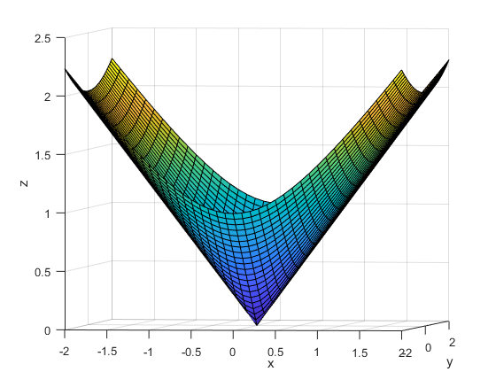
The b and gamma arguments move the cone. The A and d arguments rotate the cone and change its shape.

Algorithms

The algorithm uses an interior-point method. For details, see Second-Order Cone Programming Algorithm.

Alternative Functionality

App

The Optimize Live Editor task provides a visual interface for coneprog.

Extended Capabilities

C/C++ Code Generation

Generate C and C++ code using MATLAB® Coder™.

Usage notes and limitations:

• coneprog supports code generation using either the codegen (MATLAB Coder) function or the MATLAB^® Coder™ app. You must have a MATLAB Coder license to generate code.

• The target hardware must support standard double-precision floating-point computations.

• Code generation targets do not use the same math kernel libraries as MATLAB solvers. Therefore, code generation solutions can vary from solver solutions, especially for poorly conditioned problems.

• coneprog does not support the problem argument for code generation.

  [x,fval] = coneprog(problem) % Not supported

• All coneprog input matrices such as A, Aeq, secondordercone inputs, lb, and ub can be full or sparse. To use sparse inputs, you must enable dynamic memory allocation. See Code Generation Limitations (MATLAB Coder). Solvers have good performance with sparse inputs when the fraction of nonzero entries is small.

• Pass cone constraints as a cell array of SecondOrderConeConstraint objects, not as an array of these objects. If you have no cone constraints, pass an empty cell {}.

• The lb and ub arguments must have the same number of entries as the number of problem variables, or must be empty [].

• If your target hardware does not support infinite bounds, use optim.coder.infbound.

• For advanced code optimization involving embedded processors, you also need an Embedded Coder^® license.

• Code generation supports these options for optimoptions:

  • ConstraintTolerance

  • Display

  • LinearSolver

  • MaxIterations

  • OptimalityTolerance

• Generated code has limited error checking for options. The recommended way to update an option is to use dot notation, not optimoptions.

  opts = optimoptions("coneprog",ConstraintTolerance=1e-4);
  opts = optimoptions(opts,MaxIterations=1e4); % Not preferred
  opts.MaxIterations = 1e4; % Recommended

• coneprog supports options passed to the solver, not only options created in the code.

• If you specify an option that is not supported, the option is typically ignored during code generation. For reliable results, specify only supported options.

Version History

Introduced in R2020b

R2025a: Code generation updates

• All input matrices for coneprog code generation such as A, Aeq, lb, ub, and the inputs to secondordercone can be full or sparse.

• The new exitflag -8 applies only to code generation with sparse data.

• You can now update options using optimoptions, though the recommended way is to use dot notation.

  opts = optimoptions("coneprog",ConstraintTolerance=1e-4);
  opts = optimoptions(opts,MaxIterations=1e4); % Not preferred
  opts.MaxIterations = 1e4; % Recommended

For details, see Code Generation for coneprog Background.

R2024b: Generate code

coneprog can generate C/C++ code. For details, see Code Generation for coneprog Background and Generate Code for coneprog. To accommodate code generation, you can now pass second-order cone constraints as a cell array of SecondOrderConeConstraint objects, which is the required syntax for code generation. For more information, see Language Limitations (MATLAB Coder).

R2024a: 'normal-dense' linear solver for increased speed in dense problems

To gain speed in problems with dense data, set the LinearSolver option to 'normal-dense'. For an example, see Compare Speeds of coneprog Algorithms.

R2021a: Two coneprog lambda Structures Renamed

The coneprog lambda output argument fields lambda.eq and lambda.ineq have been renamed to lambda.eqlin and lambda.ineqlin, respectively. This change causes the coneprog lambda structure fields to have the same names as the corresponding fields in other solvers.