issatisfied

Constraint satisfaction of an optimization problem at a set of points

Since R2024a

Syntax

allsat = issatisfied(prob,pts)

allsat = issatisfied(var,pt)

allsat = issatisfied(cons,pt)

allsat = issatisfied(___,tol)

[allsat,sat] = issatisfied(___)

Description

Check constraint satisfaction.

issatisfied checks constraint satisfaction at a point or set of points for several argument types:

• A constraint object, which is an OptimizationConstraint object, an OptimizationEquality object, or an OptimizationInequality object. For a constraint object, issatisfied checks all constraints at a single point.

• A problem object, which is an OptimizationProblem object or an EquationProblem object. For a problem object that contains constraints, issatisfied can check satisfaction of multiple constraints at multiple points, and also checks the bound and integer constraints. For definitions of integer constraints, see var.

• An optimization variable, which is an OptimizationVariable object. For an optimization variable, issatisfied checks whether the variable satisfies its bound and integer constraints at a point, where the integer constraint means integer, semi-integer, or semicontinuous constraints. For definitions of integer constraints, see var.

For all argument types, issatisfied can check the constraint satisfaction to within a settable tolerance.

allsat = issatisfied(prob,pts) returns a logical vector whose length is the number of points in pts. An entry in allsat is true if all the constraints in prob are satisfied to within the default tolerance of 1e-6 for the corresponding point in pts. Otherwise, the entry is false.

allsat = issatisfied(var,pt) or allsat = issatisfied(cons,pt) returns a logical scalar indicating whether all the variables in var satisfy their bound and type constraints or whether all the constraints in cons are satisfied at the point pt.

allsat = issatisfied(___,tol), for any previous input arguments, returns true when the constraints at a point are satisfied to within the value tol, and false otherwise.

[allsat,sat] = issatisfied(___) also returns the argument sat that is an OptimizationValues object when checking problem objects, or is a logical array when checking variables or constraint objects. An OptimizationValues object contains Constraints or Equation properties that are logical indications of the constraint satisfactions for the associated constraints or equation at the corresponding evaluation point, and contains Variables properties that are logical arrays matching the size of the variables in prob and indicating the satisfaction of bound and integer constraints.

Examples

Check Constraint Satisfaction in Optimization Problem

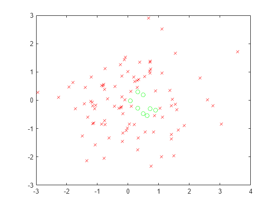
Create an optimization problem with several linear and nonlinear constraints.

x = optimvar("x");
y = optimvar("y");
obj = (10*(y - x^2))^2 + (1 - x)^2;
cons1 = x^2 + y^2 <= 1;
cons2 = x + y >= 0;
cons3 = y <= sin(x);
cons4 = 2*x + 3*y <= 2.5;
prob = optimproblem(Objective=obj);
prob.Constraints.cons1 = cons1;
prob.Constraints.cons2 = cons2;
prob.Constraints.cons3 = cons3;
prob.Constraints.cons4 = cons4;

Create 100 test points randomly.

rng default % For reproducibility
xvals = randn(1,100);
yvals = randn(1,100);

Convert the points to an OptimizationValues object for the problem, and determine where all the constraints are satisfied among the points.

vals = optimvalues(prob,x=xvals,y=yvals);
allsat = issatisfied(prob,vals);

Plot the feasible (satisfied) points with green circles and the infeasible points with red x marks.

xsat = xvals(allsat);
ysat = yvals(allsat);
xnosat = xvals(~allsat);
ynosat = yvals(~allsat);
plot(xsat,ysat,"go",xnosat,ynosat,"rx")

Check Constraint Satisfaction at a Point

Create two optimization variables and a 3-by-2 array of inequality constraints.

x = optimvar("x");
y = optimvar("y");
cons = optimconstr(3,2);
cons(1,1) = x^2 + y^2/4 <= 2;
cons(1,2) = 3*x + y <= 4;
cons(2,1) = -x - y^3 <= -3;
cons(2,2) = 2*x^2 + x*y + 4*y^2 <= 6;
cons(3,1) = 2*x + 4*x*y + y^2 <= 5;
cons(3,2) = (4 + x*y)^2 <= 24;

Check whether all constraints are satisfied at the point x = 1/2, y = -1/2.

pt.x = 1/2;
pt.y = -1/2;
allsat = issatisfied(cons,pt)

allsat = logical
   0

Not all of the constraints are satisfied. Find out which ones are satisfied.

[allsat,sat] = issatisfied(cons,pt)

allsat = logical
   0

sat = 3×2 logical array

   1   1
   0   1
   1   1

All but constraint(2,1) are satisfied.

Change Constraint Satisfaction Tolerance

Create an optimization problem with several linear and nonlinear constraints.

x = optimvar("x");
y = optimvar("y");
obj = (10*(y - x^2))^2 + (1 - x)^2;
cons1 = x^2 + y^2 <= 1;
cons2 = x + y >= 0;
cons3 = y <= sin(x);
cons4 = 2*x + 3*y <= 2.5;
prob = optimproblem(Objective=obj);
prob.Constraints.cons1 = cons1;
prob.Constraints.cons2 = cons2;
prob.Constraints.cons3 = cons3;
prob.Constraints.cons4 = cons4;

Create 100 test points randomly.

rng default % For reproducibility
xvals = randn(1,100);
yvals = randn(1,100);

Convert the points to an OptimizationValues object for the problem, and determine where all the constraints are satisfied among the points.

vals = optimvalues(prob,x=xvals,y=yvals);
allsat = issatisfied(prob,vals);

Plot the feasible (satisfied) points with green circles and the infeasible points with red x marks.

xsat = xvals(allsat);
ysat = yvals(allsat);
xnosat = xvals(~allsat);
ynosat = yvals(~allsat);
plot(xsat,ysat,"go",xnosat,ynosat,"rx")

Determine which points are feasible with respect to a tolerance of 1 rather than the default 1e-6.

tol = 1;
allsat1 = issatisfied(prob,vals,tol);

Plot the feasible (satisfied) points with green circles and the infeasible points with red x marks.

xsat1 = xvals(allsat1);
ysat1 = yvals(allsat1);
xnosat1 = xvals(~allsat1);
ynosat1 = yvals(~allsat1);
plot(xsat1,ysat1,"go",xnosat1,ynosat1,"rx")

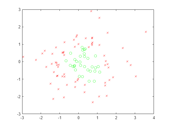
With a looser definition of constraint satisfaction, more points are feasible.

Determine Which Constraints are Satisfied

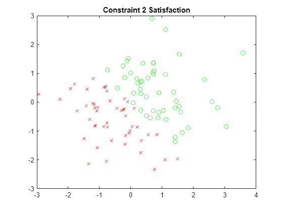
Create an optimization problem with several linear and nonlinear constraints.

x = optimvar("x");
y = optimvar("y");
obj = (10*(y - x^2))^2 + (1 - x)^2;
cons1 = x^2 + y^2 <= 1;
cons2 = x + y >= 0;
cons3 = y <= sin(x);
cons4 = 2*x + 3*y <= 2.5;
prob = optimproblem(Objective=obj);
prob.Constraints.cons1 = cons1;
prob.Constraints.cons2 = cons2;
prob.Constraints.cons3 = cons3;
prob.Constraints.cons4 = cons4;

Create 100 test points randomly.

rng default % For reproducibility
xvals = randn(1,100);
yvals = randn(1,100);

Convert the points to an OptimizationValues object for the problem.

vals = optimvalues(prob,x=xvals,y=yvals);

Evaluate the constraints at the points. issatisfied evaluates all the constraint satisfactions at all the test points simultaneously.

[~,sat] = issatisfied(prob,vals);

Plot the feasible (satisfied) points for the first constraint with green circles and the infeasible points with red x marks.

x1sat = xvals(sat.cons1);
y1sat = yvals(sat.cons1);
x1nosat = xvals(~sat.cons1);
y1nosat = yvals(~sat.cons1);
plot(x1sat,y1sat,"go",x1nosat,y1nosat,"rx")
title("Constraint 1 Satisfaction")

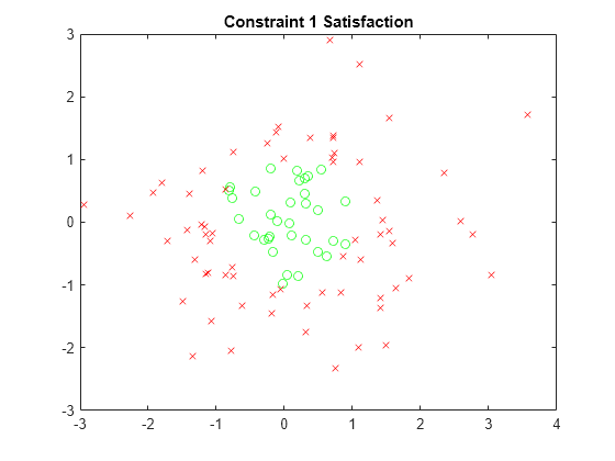
Repeat this process for the other three constraints.

x2sat = xvals(sat.cons2);
y2sat = yvals(sat.cons2);
x2nosat = xvals(~sat.cons2);
y2nosat = yvals(~sat.cons2);
plot(x2sat,y2sat,"go",x2nosat,y2nosat,"rx")
title("Constraint 2 Satisfaction")

x3sat = xvals(sat.cons3);
y3sat = yvals(sat.cons3);
x3nosat = xvals(~sat.cons3);
y3nosat = yvals(~sat.cons3);
plot(x3sat,y3sat,"go",x3nosat,y3nosat,"rx")
title("Constraint 3 Satisfaction")

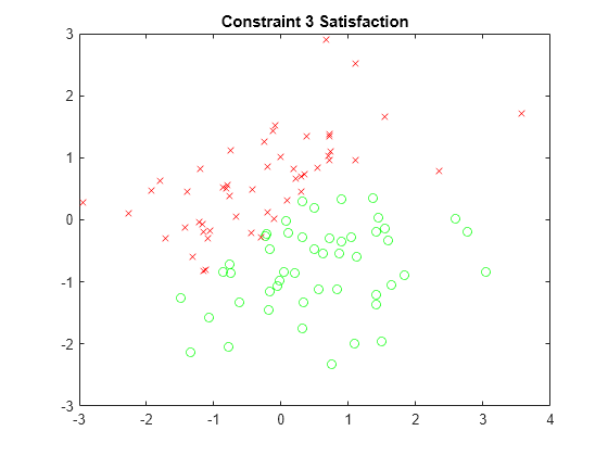
x4sat = xvals(sat.cons4);
y4sat = yvals(sat.cons4);
x4nosat = xvals(~sat.cons4);
y4nosat = yvals(~sat.cons4);
plot(x4sat,y4sat,"go",x4nosat,y4nosat,"rx")
title("Constraint 4 Satisfaction")

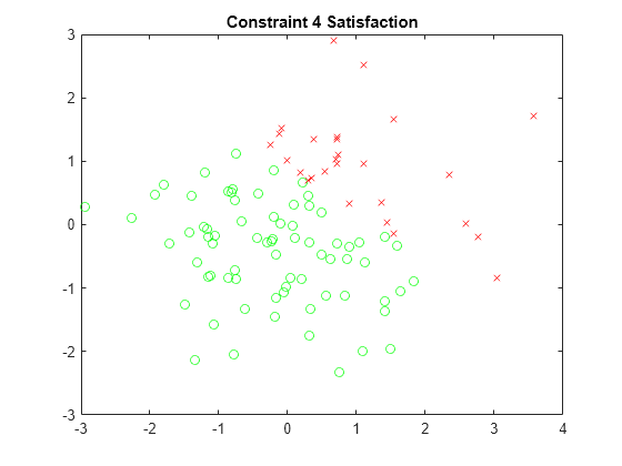
The plots show the different regions of satisfaction for each constraint.

Find Constraint, Bound, and Integer Satisfaction

Create optimization variables with bounds, integer, and semicontinuous constraints.

x = optimvar("x",LowerBound=-2,UpperBound=2,Type="integer");
y = optimvar("y",LowerBound=1/2,Type="semi-continuous");

Create an optimization problem with several linear and nonlinear constraints.

obj = (10*(y - x^2))^2 + (1 - x)^2;
cons1 = x^2 + y^2 <= 1;
cons2 = x + y >= 0;
cons3 = y <= sin(x);
cons4 = 2*x + 3*y <= 2.5;
prob = optimproblem(Objective=obj);
prob.Constraints.cons1 = cons1;
prob.Constraints.cons2 = cons2;
prob.Constraints.cons3 = cons3;
prob.Constraints.cons4 = cons4;

Create 50 test points randomly without regard to variable bounds and integer constraints, and 50 points that respect the variable bounds and integer constraints.

rng default % For reproducibility
xvals = randn(1,50);
yvals = randn(1,50);
xvals2 = randi(5,1,50) - 3; % Row vector, integer values from -2 to 2
yvals2 = abs(randn(1,50)); % Can violate the semicontinuous constraint
yvals2(yvals2 <= 1/2) = 0; % No violation of semicontinuous constraint
xvals = [xvals xvals2];
yvals = [yvals yvals2];

Convert the points to an OptimizationValues object for the problem.

vals = optimvalues(prob,x=xvals,y=yvals);

Evaluate the constraints at the points. issatisfied evaluates all the constraint satisfactions at all the test points simultaneously.

[allsat,sat] = issatisfied(prob,vals);

Find points that satisfy all of the constraints.

idx = find(allsat)

idx = 1×6

    55    58    80    93    94   100

Examine the first point in this set.

i1 = idx(1);
vals(i1)

ans = 
  OptimizationValues with properties:

   Variables properties:
            x: 1
            y: 0

   Objective properties:
    Objective: NaN

   Constraints properties:
        cons1: NaN
        cons2: NaN
        cons3: NaN
        cons4: NaN

The Variables property for y is false. Examine the x and y values of this variable.

[xvals(i1),yvals(i1)]

ans = 1×2

     1     0

The y variable does not satisfy the bound constraint, so its variable property is false. However, y does satisfy the semicontinuous constraint, so the variable satisfaction is true, as are all of the constraint satisfactions:

sat(i1)

ans = 
  OptimizationValues with properties:

   Variables properties:
            x: 1
            y: 1

   Objective properties:
    Objective: NaN

   Constraints properties:
        cons1: 1
        cons2: 1
        cons3: 1
        cons4: 1

For plots of the satisfaction of the other constraints, see Determine Which Constraints are Satisfied.

Evaluate Expressions in Equation

Create a set of equations in two optimization variables.

x = optimvar("x");
y = optimvar("y");
prob = eqnproblem;
prob.Equations.eq1 = x^2 + y^2/4 == 2;
prob.Equations.eq2 = x^2/4 + 2*y^2 == 2;

Solve the system of equation starting from $$x=1,y=1/2$$.

x0.x = 1;
x0.y = 1/2;
sol = solve(prob,x0)

Solving problem using fsolve.

Equation solved.

fsolve completed because the vector of function values is near zero
as measured by the value of the function tolerance, and
the problem appears regular as measured by the gradient.

<stopping criteria details>

sol = struct with fields:
    x: 1.3440
    y: 0.8799

Evaluate the equations at the points x0 and sol.

vars = optimvalues(prob,x=[x0.x sol.x],y=[x0.y sol.y]);
vals = evaluate(prob,vars)

vals = 
  1×2 OptimizationValues vector with properties:

   Variables properties:
      x: [1 1.3440]
      y: [0.5000 0.8799]

   Equation properties:
    eq1: [0.9375 8.4322e-10]
    eq2: [1.2500 6.7431e-09]

The first point, x0, has nonzero values for both equations eq1 and eq2. The second point, sol, has nearly zero values of these equations, as expected for a solution.

Find the degree of equation satisfaction using issatisfied.

[satisfied details] = issatisfied(prob,vars)

satisfied = 1×2 logical array

   0   1

details = 
  1×2 OptimizationValues vector with properties:

   Variables properties:
      x: [1 1]
      y: [1 1]

   Equation properties:
    eq1: [0 1]
    eq2: [0 1]

The first point, x0, is not a solution, and satisfied is 0 for that point. The second point, sol, is a solution, and satisfied is 1 for that point. The equation properties show that neither equation is satisfied at the first point, and both are satisfied at the second point.

Input Arguments

prob — Object for evaluation

OptimizationProblem object | EquationProblem object

Object for evaluation, specified as an OptimizationProblem object or an EquationProblem object. The issatisfied function evaluates the objectives and constraints in the properties of prob at the points in pts.

Example: prob = optimproblem(Objective=obj,Constraints=constr)

pts — Points to evaluate for prob

structure | OptimizationValues object

Points to evaluate for prob, specified as a structure or an OptimizationValues object.

• The field names in pts must match the corresponding variable names in the objective and constraint expressions in prob.

• The values in pts must be numeric arrays of the same size as the corresponding variables in prob.

Note

Currently, pts can be an OptimizationValues object only when prob is an EquationProblem object or an OptimizationProblem object.

If you use a structure for pts, then pts can contain only one point. In other words, if you want to evaluate multiple points simultaneously, pts must be an OptimizationValues object.

Example: pts = optimvalues(prob,x=xval,y=yval)

cons — Constraint

OptimizationConstraint object | OptimizationEquality object | OptimizationInequality object

Constraint, specified as an OptimizationConstraint object, an OptimizationEquality object, or an OptimizationInequality object. issatisfied applies to these constraint objects only for a point specified as a structure, not as an OptimizationValues object.

Example: cons = expr1 <= expr2, where expr1 and expr2 are optimization expressions

var — Optimization variable

OptimizationVariable object

Optimization variable, specified as an OptimizationVariable object. issatisfied computes bound and integer constraint violations as follows.

Variable Type	Infeasibility for Bounds and Type
Continuous	max(0,lb - x,x - ub)
Integer	max(0,lb - x,x - ub,abs(x - round(x)))
Semi-continuous	min(max(0,lb - x,x - ub),abs(x))
Semi-integer	min(max(0,lb - x,x - ub,abs(x - round(x))),abs(x))

Example: var = optimvar("var",LowerBound=0,UpperBound=10.5)

pt — Values of variables in expression

structure

Values of the variables in an expression, specified as a structure. The structure pt has the following requirements:

• All variables in expr must match field names in pt.

• The values of the matching field names must be numeric.

• The sizes of the fields in pt must match the sizes of the corresponding variables in expr.

For example, pt can be the solution to an optimization problem, as returned by solve.

Example: pt.x = 3, pt.y = -5

Data Types: struct

tol — Tolerance for constraint satisfaction

1e-6 (default) | nonnegative scalar

Tolerance for constraint satisfaction, specified as a nonnegative scalar. A constraint is considered to be satisfied if it evaluates to no more than tol. Otherwise, the constraint is unsatisfied.

For example, if c(x) is a nonlinear inequality constraint function, then when c(pt) ≤ tol, issatisfied returns true for that constraint at the point pt. Similarly, if ceq(x) is a nonlinear equality constraint function, then when abs(ceq(pt)) ≤ tol, issatisfied returns true for that constraint at the point pt.

Data Types: double

Output Arguments

allsat — Indication that all constraints are satisfied

logical vector

Indication that all constraints are satisfied at the given points, returned as a logical row vector. allsat(i) corresponds to the query point pts(i). The returned value is true if all values of the constraint functions are no more than tol. If pts is a structure, then allsat is a logical scalar.

sat — Indication that a constraint is satisfied at the given points

OptimizationValues vector | logical array

Indication that a constraint is satisfied at the given points, returned as an OptimizationValues vector for an OptimizationProblem or EquationProblem object, or a logical array for a variable or constraint object.

For a problem object, sat is an OptimizationValues object, whose length equals the number of points in pt or pts. sat(i) contains bound/type/constraint satisfaction information for the ith point. In sat(i),

• The Variables properties are logical arrays matching the size of the variables in prob

• The Constraints or Equations properties match the size of the constraints or equations in prob

For a problem object, index into sat using the constraint or equation names. For example, if pts is an OptimizationValues object with N = 5 points, and con is a constraint expression of size 2-by-3, then sat.con has size 2-by-3-by-5. The entries are true for satisfied constraints to within the tolerance tol.

For a constraint object (OptimizationConstraint, OptimizationEquality, or OptimizationInequality), the size of sat is the same as the size of the associated constraint.

For a variable object, the size of sat is the same as the size of the variable.

More About

Constraint Expression Values

For a constraint expression at a point pt:

• If the constraint is L <= R, the constraint value is evaluate(L,pt) – evaluate(R,pt).

• If the constraint is L >= R, the constraint value is evaluate(R,pt) – evaluate(L,pt).

• If the constraint is L == R, the constraint value is abs(evaluate(L,pt) – evaluate(R,pt)).

Generally, a constraint is considered to be satisfied (or feasible) at a point if the constraint value is less than or equal to a tolerance.

Tips

The toolbox has three functions to compute the feasibility of points.

• infeasibility — Compute the numeric violation value of an OptimizationVariable (with respect to its bound and type constraints) or an OptimizationConstraint at a point.

• issatisfied — Check if the infeasibility of an OptimizationVariable or an OptimizationConstraint or components of an OptimizationProblem or EquationProblem at a point exceed some threshold.

• evaluate — Compute the value of an OptimizationVariable, OptimizationExpression, OptimizationConstraint, or components of an OptimizationProblem or EquationProblem at a point.

Version History

Introduced in R2024a

R2026a: Check bounds and variable types

issatisfied now checks satisfaction with respect to variable bounds and integer constraints as well as satisfaction of linear and nonlinear constraints. If a point does not satisfy the bounds or integer constraints to within the tolerance, issatisfied returns false. issatisfied computes satisfaction with respect to bounds and integer constraints as described in var.

issatisfied now sets the Variables property of each element of the sat output to a logical value representing the satisfaction of that element with respect to bounds and integer constraints. Previously, the Variables property held the variable values in the pts input.

R2024b: Evaluate expressions in more objects

The issatisfied function now applies to the following objects:

• EquationProblem

• OptimizationConstraint

• OptimizationEquality

• OptimizationInequality

For an example, see Evaluate Expressions in Equation.

R2024a: Evaluate satisfaction in optimization problems at multiple points

The issatisfied function now applies to objective and constraint expressions in OptimizationProblem objects. If the evaluation points are passed as an OptimizationValues object, then the function determines satisfaction at all points in the object. For an example, see Determine Which Constraints are Satisfied.