What Is Parallel Computing in Optimization Toolbox?
Parallel Optimization Functionality
Parallel computing is the technique of using multiple processors on a single problem. The reason to use parallel computing is to speed computations.
The following Optimization Toolbox™ solvers can automatically distribute the numerical estimation of gradients of objective functions and nonlinear constraint functions to multiple processors:
fminconfminuncfgoalattainfminimaxfsolvelsqcurvefitlsqnonlin
These solvers use parallel gradient estimation under the following conditions:
You have a license for Parallel Computing Toolbox™ software.
The option
SpecifyObjectiveGradientis set tofalse, or, if there is a nonlinear constraint function, the optionSpecifyConstraintGradientis set tofalse. Sincefalseis the default value of these options, you don't have to set them; just don't set them both totrue.Parallel computing is enabled with
parpool, a Parallel Computing Toolbox function.The option
UseParallelis set totrue. The default value of this option isfalse.
When these conditions hold, the solvers compute estimated gradients in parallel.
Note
Even when running in parallel, a solver occasionally calls the objective and nonlinear constraint functions serially on the host machine. Therefore, ensure that your functions have no assumptions about whether they are evaluated in serial or parallel.
Parallel Estimation of Gradients
One solver subroutine can compute in parallel automatically: the subroutine that estimates the gradient of the objective function and constraint functions. This calculation involves computing function values at points near the current location x. Essentially, the calculation is
where
f represents objective or constraint functions
ei are the unit direction vectors
Δi is the size of a step in the ei direction
To estimate ∇f(x) in parallel, Optimization Toolbox solvers distribute the evaluation of (f(x + Δiei) – f(x))/Δi to extra processors.
Parallel Central Differences
You can choose to have gradients estimated by central finite differences instead of the default forward finite differences. The basic central finite difference formula is
This takes twice as many function evaluations as forward finite differences, but is usually much more accurate. Central finite differences work in parallel exactly the same as forward finite differences.
Enable central finite differences by using optimoptions
to set the FiniteDifferenceType option to
'central'. To use forward finite differences, set the
FiniteDifferenceType option to
'forward'.
Nested Parallel Functions
Solvers employ the Parallel Computing Toolbox function parfor (Parallel Computing Toolbox) to perform parallel
estimation of gradients. parfor does not work in parallel when
called from within another parfor loop. Therefore, you cannot
simultaneously use parallel gradient estimation and parallel functionality within
your objective or constraint functions.
Note
The documentation recommends not to use parfor or
parfeval when calling Simulink®; see Using sim Function Within parfor (Simulink). Therefore, you might
encounter issues when optimizing a Simulink simulation in parallel using a solver's built-in parallel functionality. For
an example showing how to optimize a Simulink model with several Global Optimization Toolbox solvers, see Optimize Simulink Model in Parallel (Global Optimization Toolbox).
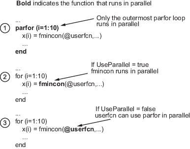
Suppose, for example, your objective function userfcn calls
parfor, and you want to call fmincon
in a loop. Suppose also that the conditions for parallel gradient evaluation of
fmincon, as given in Parallel Optimization Functionality, are satisfied. When parfor Runs In Parallel shows three cases:
The outermost loop is
parfor. Only that loop runs in parallel.The outermost
parforloop is infmincon. Onlyfminconruns in parallel.The outermost
parforloop is inuserfcn.userfcncan useparforin parallel.
When parfor Runs In Parallel
See Also
Using Parallel Computing in Optimization Toolbox | Improving Performance with Parallel Computing | Minimizing an Expensive Optimization Problem Using Parallel Computing Toolbox