Accelerate Seismic Migration Using CUDA Code
R2026bThis example shows how to accelerate seismic reverse time migration (RTM) by implementing parts of the algorithm in CUDA® code and running them on a GPU.
Seismic migration converts time-domain seismic records from the surface into their correct spatial positions. RTM produces an accurate representation of the subsurface but is computationally expensive.
This example shows how to:
Perform RTM on CPU.
Accelerate the RTM algorithm by implementing key steps in CUDA code and running them on a GPU.
Reverse Time Migration
Reverse time migration comprises three main steps [1]:
Starting with a velocity model, simulate the propagation of a downward-propagating seismic wave generated by a source at the surface and record the waves reflected back to the surface. You simulate the wave by numerically solving the wave equation with absorbing boundary conditions at the edges. This is referred to as forward migration.
Starting from the recorded waves at the surface from the forward migration, propagate these upward-propagating waves backwards through time.
Correlate the downward-propagating wavefield with the upward-propagating wavefield at each timestep. As the downward-propagating wavefield and the upward-propagating are coincident at reflecting velocity boundaries, the correlation shows the depths of these boundaries and constructs an image of the subsurface.
The function cpuRTM is defined at the end of this example, and performs these steps on the CPU in single precision. It performs the migration process repeatedly across several horizontal positions that represent the locations of seismic sources.
Load the example data. The data is from the 2004 BP velocity estimation benchmark model [2]. It was synthetically generated using a mixed-domain 2-D finite-difference acoustic modeling and is a challenging benchmark for seismic processing techniques.
filename = "vel_z6.25m_x12.5m_exact.segy";
if ~isfile(filename)
    segYLocation = "http://s3.amazonaws.com/open.source.geoscience/open_data/bpvelanal2004/vel_z6.25m_x12.5m_exact.segy.gz";
    gunzip(segYLocation);

    readmeLocation = "https://s3.amazonaws.com/open.source.geoscience/open_data/bpvelanal2004/2004_Benchmark_READMES.pdf";
    websave("2004_Benchmark_READMES.pdf",readmeLocation);
end

addpath("fileReader")
V = SegYFileReader(filename{1},true,false);
V = V(:,:);
V = single(V);
Specify the parameters of the model.
nz = 1911;          % depth samples
dz = 6.25;          % depth spacing (m)
nx = 5395;          % surface samples
dx = 12.5;          % surface spacing (m)
Plot the starting velocity model. This model is a high-resolution, synthetically-generated map of the speed of seismic waves through the subsurface. In a real application, this would be a lower-resolution, estimated velocity model.
figure
imagesc((0:nx-1)*dx,(0:nz-1)*dz,V)
axis equal tight
colormap(seismic)
title("Velocity Model")
c = colorbar;
c.Label.String = "Velocity (m/s)";
xlabel("Distance (m)")
ylabel("Depth (m)")
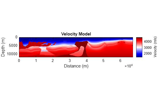
To run this example in a reasonable time, extract a subset of the data and downsample. The extracted subset includes a tooth-shaped salt formation.
z = single((0:nz-1)*dz);
x = single((0:nx-1)*dx);

dz = single(diff(z(1:2)));

idx = 2200:3400;
x = x(idx);
V = V(:,idx);

[rows,cols] = size(V);
new_rows = 120;
new_cols = 120;

row_idx = round(linspace(1, rows, new_rows));
col_idx = round(linspace(1, cols, new_cols));

V = V(row_idx,col_idx);
figure
imagesc(x,z,V)
axis equal tight
colormap(seismic)
title("Velocity Model")
c = colorbar;
c.Label.String = "Velocity (m/s)";
xlabel("Distance (m)")
ylabel("Depth (m)")
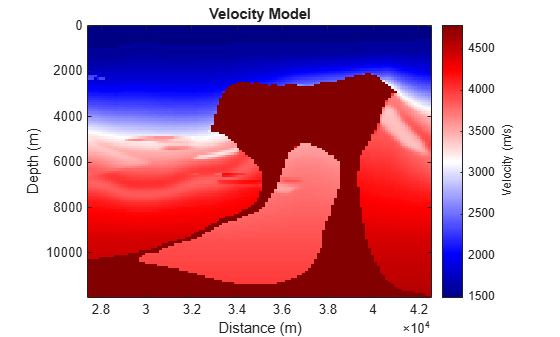
Specify the size of the time step to use for solving wave equation. The size of the time step must satisfy the Courant–Friedrichs–Lewy condition for calculations to be stable, that is, the size of the time steps must be less than the time it takes for a wave to travel between adjacent grid points.
dt = single(0.9*min(min(dz./V/sqrt(2))));
Run the CPU RTM and time the execution using tic and toc.
tic
StackedCPU = cpuRTM(V,x,z,dt);
tCPU = toc
tCPU =
414.9007
Accelerate RTM Using Custom CUDA Kernels
Running MATLAB® functions on a GPU using gpuArray can speed up your code. To further improve performance, you can write custom CUDA code and call it from MATLAB. Custom CUDA code gives you access to advanced features, such as dynamic memory allocation, fine-grained control over kernel launches, and cooperative groups. For more information about running your own CUDA code in MATLAB, see Run MEX Functions Containing CUDA Code.
The gpuRTMSingle function, defined at the end of this example, uses both gpuArray and CUDA code to accelerate the code in the following ways:
When the input velocity model
Vis agpuArray, the function performs the preprocessing steps (the steps before the forward and reverse migration processes) on the GPU. These include preallocating arrays and determining the number of time steps to use for the forward and reverse migration.The function uses two MEX files that perform the forward and reverse migration. Each mex file contains a kernel that numerically solves the wave equation over multiple time steps on the GPU. The kernel uses cooperative groups of threads to synchronize across all thread blocks in a grid. Solving across all of the time steps in a single kernel reduces the number of kernels launched by the GPU, reducing kernel launch overhead and memory traffic.
Compile the forward and reverse migration MEX files.
forwardSingleCU = "fm2d_kernel_time_integrated_single_gridstride.cu";
mexcuda(forwardSingleCU,"-output","forwardSingle")
Building with 'NVIDIA CUDA Compiler'.
MEX completed successfully.
reverseSingleCU = "rtm2d_kernel_timeloop_single_gridstride.cu";
mexcuda(reverseSingleCU,"-output","reverseSingle")
Building with 'NVIDIA CUDA Compiler'.
MEX completed successfully.
Check whether a GPU is available.
gpu = gpuDevice;
disp(gpu.Name + " GPU detected and available.")
NVIDIA RTX A5000 GPU detected and available.
Convert the input data to a gpuArray and run the GPU RTM. Time the execution using tic and toc.
VGPU = gpuArray(V);
tic
StackedMexcuda = gpuRTMSingle(VGPU,x,z,dt);
tGPU = toc
tGPU =
4.0451
Compare Results
Plot the results from the CPU and GPU calculations to check that they both highlight the reflecting surfaces and are consistent with each other. The results differ slightly due to differences in how CPUs and GPUs handle floating-point numbers, and the differences compound when solving the wave equation over many time steps.
figure
tiledlayout(1,2)

nexttile
imagesc(x,z,diff(StackedCPU(1:end-20,21:end-20),2,1))
ax = gca;
ax.ColorScale = "log";
axis equal tight
title("CPU")
xlabel("Distance (m)")
ylabel("Depth (m)")

nexttile
imagesc(x,z,diff(StackedMexcuda(1:end-20,21:end-20),2,1))
ax = gca;
ax.ColorScale = "log";
axis equal tight
title("GPU using \fontname{monospace}mexcuda")
xlabel("Distance (m)")
ylabel("Depth (m)")
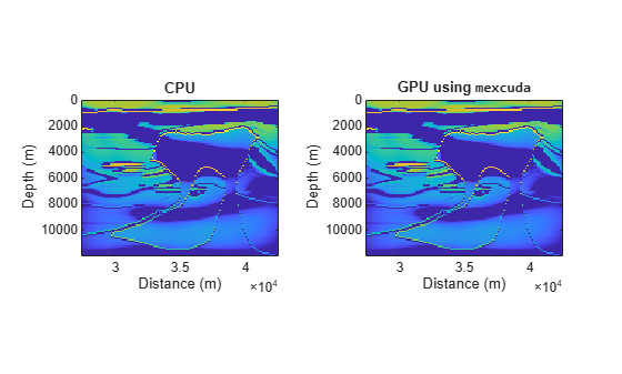
Compare the execution times of the CPU and GPU mexcuda implementations.
figure
b = bar(["CPU","GPU via \fontname{monospace}mexcuda"],[tCPU tGPU]);
b.Labels = round(b.YData,1);
ylabel("Execution Time (s)")
xlabel("Execution Environment")
title("RTM Performance Comparison")
grid on
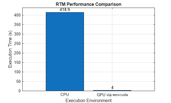
The GPU implementation using mexcuda is significantly faster.
When you apply the techniques described in this example to your own code, the performance improvement will strongly depend on your hardware and on the code you run.
References
[1] Baysal, Edip, et al. “Reverse Time Migration.” Geophysics, vol. 48, no. 11, Nov. 1983, pp. 1514–24. DOI.org (Crossref), https://doi.org/10.1190/1.1441434.
[2] Billette, Frederic, and Sverre Brandsberg-Dahl. The 2004 BP Velocity Benchmark. 2005. EAGE. EAGE, Expanded Abstracts, 67th Annual International Meeting
Supporting Functions
RTM on CPU
The cpuRTM function performs reverse time migration entirely on the CPU. It takes a 2-D velocity model V, spatial coordinate vectors x and z, and a time step dt as inputs, and returns the stacked cross-correlation image of the subsurface.
function stacked = cpuRTM(V,x,z,dt)
% Calculate step size parameters.
[nz,nx] = size(V);
dx = single(diff(x(1:2)));
dz = single(diff(z(1:2)));

% Determine the number of time samples to use from wave travel time to depth and back to
% surface.
vmin = min(V(:));
nt = single(round((sqrt((dx*nx)^2 + (dz*nx)^2)*2/vmin/dt + 1)));

% Add a 20 node wide region around the model for applying absorbing boundary conditions.
V = [repmat(V(:,1),1,20) V repmat(V(:,end),1,20)];
V(end+1:end+20,:) = repmat(V(end,:),20,1);

% Define frequency parameter for ricker wavelet.
f  = 20;

stacked = zeros(nz+20,nx+40,"single");

% Shot loop
for ixs = 21:nx+20
    % Initial wavefield - initial condition of a Ricker wavelet at
    % surface.
    rw = ricker(f,nz+40,dt,dt*ixs,0);
    rw = single(rw(1:nz+20,:));

    % Run forward migration, then reverse migration using the recorded surface data.
    [data,snapshot] = fm2d(V,rw,nz,dz,nx,dx,nt,dt);
    [~,snapshotRTM] = rtm2d(V,data,nz,dz,nx,dx,nt,dt);

    % Flip the time axis so forward and reverse snapshots are aligned.
    snapshotRTM = flip(snapshotRTM,3);

    % Correlate the forward and reverse wavefields to image reflecting boundaries.
    M = sum(snapshot .* snapshotRTM,3);

    % Accumulate across shots to reinforce true reflectors and suppress noise.
    stacked = M + stacked;

end
end
RTM on GPU
The gpuRTMSingle function performs reverse time migration using GPU-accelerated MEX files compiled with mexcuda. It takes the same inputs as cpuRTM — a 2-D velocity model V (as a gpuArray), spatial coordinate vectors x and z, and a time step dt, and returns the stacked cross-correlation image.
function stacked = gpuRTMSingle(V,x,z,dt)
% Calculate step size parameters.
[nz,nx] = size(V);
dx = single(diff(x(1:2)));
dz = single(diff(z(1:2)));

% Determine time samples nt from wave travel time to depth and back to
% surface.
vmin = min(V(:));
nt = single(round((sqrt((dx*nx)^2 + (dz*nx)^2)*2/vmin/dt + 1)));

% Add region around model for applying absorbing boundary conditions (20
% nodes wide).
V = [repmat(V(:,1),1,20) V repmat(V(:,end),1,20)];
V(end+1:end+20,:) = repmat(V(end,:),20,1);

% Define frequency parameter for ricker wavelet.
f  = 20;

% Specify the absorbing boundary and the finite-difference coefficients.
[nzV,nxV] = size(V);
izBC = single(1:20);
boundary = gpuArray(single((exp(-( (0.015*(20-izBC)).^2 ) )).^10));
a = gpuArray(single((V*dt/dx).^2));
b = single(2)-single(4)*a;

stacked = zeros(nz+20,nx+40,like=V);

% Shot loop
for ixs = 21:nx+20
    % Set initial condition of a mexihat wavelet at
    % surface.
    rw = ricker(f,nz+40,dt,dt*ixs,0);
    rw = gpuArray(single(rw(1:nz+20,:)));

    % Run forward migration, then reverse migration using the recorded surface data.
    [data,snapshot] = forwardSingle(rw,a,b,boundary,nt);
    [~,snapshotRTM] = rtm2dGPUSingle(data);

    % Flip the time axis so forward and reverse snapshots are aligned.
    snapshotRTM = flip(snapshotRTM,3);

    % Correlate the forward and reverse wavefields to image reflecting boundaries.
    M = sum(snapshot .* snapshotRTM,3);

    % Accumulate across shots to reinforce true reflectors and suppress noise.
    stacked = M + stacked;

end

    function [model,snapshot] = rtm2dGPUSingle(data)
        [~,ntR] = size(data);

        % Initialize single-precision wavefields.
        fdm1 = gpuArray(single([data(:,ntR)'; zeros(nzV-1,nxV)]));
        fdm2 = gpuArray(single([data(:,ntR-1)'; zeros(nzV-1,nxV)]));
        fdm3 = gpuArray(single([data(:,ntR-2)'; zeros(nzV-1,nxV)]));

        % Convert data to gpuArray.
        dataGPU = gpuArray(data);

        % Call reverse MEX function.
        [model,snapshot] = reverseSingle(fdm1,fdm2,fdm3,boundary,a,b,nzV,nxV,dataGPU,ntR);
    end
end

