plotSummary
Description
plotSummary( creates a figure
containing six plots with the battery P2D modeling results: the terminal voltage,
concentration of Li-ion in the liquid electrolyte, electric potential in the liquid
electrolyte, concentration of Li-ion in the solid active material particles in both the
anode and cathode, electric potential in the solid active material particles in both the
anode and cathode, and the ionic flux.results)
Examples
Solve a Li-Ion battery electrochemistry problem by using a pseudo-2D battery model.
Both the anode and cathode materials require the open circuit potential specification, which determines the voltage profile of the battery during charging and discharging. The open circuit potential is a voltage of electrode material as a function of the stoichiometric ratio, which is the ratio of intercalated lithium in the solid to maximum lithium capacity. You can specify this ratio by interpolating the gridded data set.
sNorm = linspace(0.025, 0.975, 39);
ocp_n_vec = [.435;.325;.259;.221;.204; ...
    .194;.179;.166;.155;.145; ...
    .137;.131;.128;.127;.126; ...
    .125;.124;.123;.122;.121; ...
    .118;.117;.112;.109;.105; ...
    .1;.098;.095;.094;.093; ...
    .091;.09;.089;.088;.087; ...
    .086;.085;.084;.083];
ocp_p_vec = [3.598;3.53;3.494;3.474; ...
    3.46;3.455;3.454;3.453; ...
    3.4528;3.4526;3.4524;3.452; ...
    3.4518;3.4516;3.4514;3.4512; ...
    3.451;3.4508;3.4506;3.4503; ...
    3.45;3.4498;3.4495;3.4493; ...
    3.449;3.4488;3.4486;3.4484; ...
    3.4482;3.4479;3.4477;3.4475; ...
    3.4473;3.447;3.4468;3.4466; ...
    3.4464;3.4462;3.4458];

anodeOCP = griddedInterpolant(sNorm,ocp_n_vec,"linear","nearest");
cathodeOCP = griddedInterpolant(sNorm,ocp_p_vec,"linear","nearest");
Create objects that specify the active materials for the anode and cathode.
anodeMaterial = batteryActiveMaterial( ...
    ParticleRadius=5E-6, ...
    MaximumSolidConcentration=30555, ...
    VolumeFraction=0.58, ...
    DiffusionCoefficient=3.0E-15, ...
    ReactionRate=8.8E-11, ...
    OpenCircuitPotential=@(st_ratio) anodeOCP(st_ratio), ...
    StoichiometricLimits=[0.0132 0.811]);

cathodeMaterial = batteryActiveMaterial(...
    ParticleRadius=5E-8, ...
    MaximumSolidConcentration=22806, ...
    VolumeFraction=0.374, ...
    DiffusionCoefficient=5.9E-19, ...
    ReactionRate=2.2E-13, ...
    OpenCircuitPotential=@(st_ratio) cathodeOCP(st_ratio), ...
    StoichiometricLimits=[0.035 0.74]);
Next, create objects that specify both electrodes.
anode = batteryElectrode(...
    Thickness=34E-6, ...
    Porosity=0.3874, ...
    BruggemanCoefficient=1.5, ...
    ElectricalConductivity=100, ...
    ActiveMaterial=anodeMaterial);

cathode = batteryElectrode(...
    Thickness=80E-6, ...
    Porosity=0.5725, ...
    BruggemanCoefficient=1.5, ...
    ElectricalConductivity=0.5, ...
    ActiveMaterial=cathodeMaterial);
Create an object that specifies the properties of the separator.
separator = batterySeparator(...
    Thickness=25E-6, ...
    Porosity=0.45, ...
    BruggemanCoefficient=1.5);
Create an object that specifies the properties of the electrolyte.
electrolyte = batteryElectrolyte(...
    DiffusionCoefficient=2E-10, ...
    TransferenceNumber=0.363, ...
    IonicConductivity=0.29);
Create an object that specifies the initial conditions of the battery.
ic = batteryInitialConditions(...
    ElectrolyteConcentration=1000, ...
    StateOfCharge=0.05, ...
    Temperature=298.15);
Create an object that specifies the properties of the battery cycling step.
cycling = batteryCyclingStep(...
    NormalizedCurrent=0.5, ...
    CutoffTime=100, ...
    CutoffVoltageUpper=4.2, ...
    OutputTimeStep=10);
Create a model for the battery P2D analysis.
model = batteryP2DModel(...
    Anode=anode, ...
    Separator=separator, ...
    Cathode=cathode, ...
    Electrolyte=electrolyte, ...
    InitialConditions=ic, ...
    CyclingStep=cycling);
Set the maximum step size for the internal solver to 2.
model.SolverOptions.MaxStep = 2;
Solve the model using the solve function. The resulting object contains the concentration of Li-ion and electric potential in solid active material particles in both the anode and cathode, as well as in the liquid electrolyte. The object also contains the voltage at the battery terminals, ionic flux, solution times, and mesh.
results = solve(model)
results =
  batteryP2DResults with properties:

                SolutionTimes: [11×1 double]
              TerminalVoltage: [11×1 double]
            NormalizedCurrent: [11×1 double]
          LiquidConcentration: [11×49 double]
               SolidPotential: [11×49 double]
              LiquidPotential: [11×49 double]
                    IonicFlux: [11×49 double]
    AverageSolidConcentration: [11×49 double]
    SurfaceSolidConcentration: [11×49 double]
           SolidConcentration: [11×7×49 double]
                         Mesh: [1×1 batteryMesh]
Visualize the results.
plotSummary(results)
![Figure contains 6 axes objects. Axes object 1 with title Terminal Voltage [V], xlabel Time [s] contains an object of type line. Axes object 2 with title Normalized Current, xlabel Time [s] contains an object of type line. Axes object 3 with title Liquid Concentration [mol/m Cubed baseline ], xlabel Thickness [m] contains 7 objects of type line, rectangle. Axes object 4 with title Normalized Average Solid Concentration, xlabel Thickness [m] contains 7 objects of type line, rectangle. Axes object 5 with title Liquid Potential [V], xlabel Thickness [m] contains 7 objects of type line, rectangle. Axes object 6 with title Solid Potential [V], xlabel Thickness [m] contains 7 objects of type line, rectangle. These objects represent 0, 30, 60, 100.](../../examples/pde/win64/SolveModelForBatteryP2DAnalysisExample_01.png)
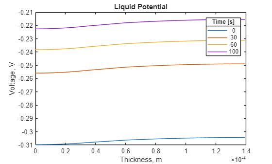
To see more details of the liquid potential distribution, plot it separately. Use the same four solution times.
figure
for i = [1 4 7 11]
plot(results.Mesh.Nodes, ...
results.LiquidPotential(i,:))
    hold on
end
title("Liquid Potential")
xlabel("Thickness, m")
ylabel("Voltage, V")
lgd = legend(num2str(results.SolutionTimes([1;4;7;11])));
lgd.Title.String = "Time [s]";
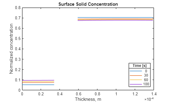
Plot the surface solid concentration distribution for the same four solution times.
figure
for i = [1 4 7 11]
plot(results.Mesh.Nodes, ...
results.SurfaceSolidConcentration(i,:))
    hold on
end
title("Surface Solid Concentration")
xlabel("Thickness, m")
ylabel("Normalized concentration")
lgd = legend(num2str(results.SolutionTimes([1;4;7;11])));
lgd.Location = "southeast";
lgd.Title.String = "Time [s]";
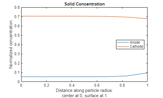
For the final solution time, 100s, plot the solid concentration along the particle radius at two locations corresponding approximately to the middle of the anode and the middle of the cathode.
figure
Rfinal = results.SolidConcentration(end,:,:);
Nr = size(results.SolidConcentration,2);
for x = [results.Mesh.AnodeNodes(ceil(end/2)) ...
         results.Mesh.CathodeNodes(ceil(end/2))]
    Rr = Rfinal(:,:,x);
plot((0:Nr-1).'/(Nr-1),Rr(:))
    hold on
end
title("Solid Concentration")
xlabel({"Distance along particle radius:";"center at 0, surface at 1"})
ylabel("Normalized concentration")
legend("Anode","Cathode",Location="east");
Input Arguments
Output Arguments
Version History
Introduced in R2026a