specifyCoefficients
Specify coefficients in PDE model
Syntax
Description
Examples
Specify the coefficients for Poisson's equation .
solvepde addresses equations of the form
.
Therefore, the coefficients for Poisson's equation are , , , , . Include these coefficients in a PDE model of the L-shaped membrane.
model = createpde();
geometryFromEdges(model,@lshapeg);
specifyCoefficients(model,m=0,...
                          d=0,...
                          c=1,...
                          a=0,...
                          f=1);
Specify zero Dirichlet boundary conditions, mesh the model, and solve the PDE.
applyBoundaryCondition(model,"dirichlet", ...
                             Edge=1:model.Geometry.NumEdges, ...
                             u=0,InternalBC=true);
generateMesh(model,Hmax=0.25);
results = solvepde(model);
View the solution.
pdeplot(model,XYData=results.NodalSolution)
axis equal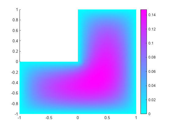
Specify coefficients for Poisson's equation in 3-D with a nonconstant source term, and obtain the coefficient object.
The equation coefficients are , , , . For the nonconstant source term, take .
f = @(location,state)location.y.^2.*tanh(location.z)/1000;
Set the coefficients in a 3-D rectangular block geometry.
model = createpde();
importGeometry(model,"Block.stl");
CA = specifyCoefficients(model,"m",0,...
                               "d",0,...
                               "c",1,...
                               "a",0,...
                               "f",f)
CA =
  CoefficientAssignment with properties:

    RegionType: 'cell'
      RegionID: 1
             m: 0
             d: 0
             c: 1
             a: 0
             f: @(location,state)location.y.^2.*tanh(location.z)/1000
Set zero Dirichlet conditions on face 1, mesh the geometry, and solve the PDE.
applyBoundaryCondition(model,"dirichlet","Face",1,"u",0);
generateMesh(model);
results = solvepde(model);
View the solution on the surface.
pdeplot3D(model,"ColorMapData",results.NodalSolution)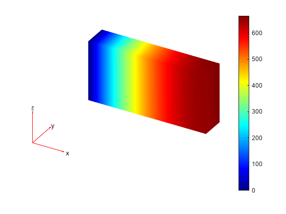
Create a scalar PDE model with the L-shaped membrane as the geometry. Plot the geometry and subdomain labels.
model = createpde();
geometryFromEdges(model,@lshapeg);
pdegplot(model,FaceLabels="on")
axis equal
ylim([-1.1,1.1])

Set the c coefficient to 1 in all domains, but the f coefficient to 1 in subdomain 1, 5 in subdomain 2, and -8 in subdomain 3. Set all other coefficients to 0.
specifyCoefficients(model,m=0,d=0,c=1,a=0,f=1,Face=1);
specifyCoefficients(model,m=0,d=0,c=1,a=0,f=5,Face=2);
specifyCoefficients(model,m=0,d=0,c=1,a=0,f=-8,Face=3);
Set zero Dirichlet boundary conditions to all edges. Create a mesh, solve the PDE, and plot the result.
applyBoundaryCondition(model,"dirichlet", ...
                             Edge=1:model.Geometry.NumEdges, ...
                             u=0,InternalBC=true);
generateMesh(model,Hmax=0.25);
results = solvepde(model);
pdeplot(model,XYData=results.NodalSolution)
axis equal

Perform transient analysis of a simple cantilever beam with and without damping. To include damping in the analysis, specify nonzero m and d coefficients.
Create a geometry representing a cantilever beam. The beam is 5 inches long and 0.1 inch thick.
height = 0.1;
width = 5;
gm = [3;4;0;width;width;0;0;0;height;height];
g = decsg(gm,'S1',('S1')');
Create a PDEModel object with two independent variables, and include a geometry in the model.
model = createpde(2);
geometryFromEdges(model,g);
Plot the geometry with edge labels.
pdegplot(model,EdgeLabels="on")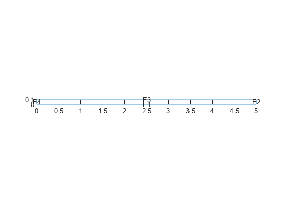
Specify that the left edge of the beam is a fixed boundary.
applyBoundaryCondition(model,"dirichlet",Edge=4,u=[0,0]);Specify Young's modulus, Poisson's ratio, and the mass density of the beam assuming that it is made of steel.
E = 3.0e7;
nu = 0.3;
rho = 0.3/386;
Specify the PDE coefficients for the undamped model by setting the d coefficient to 0.
G = E/(2.*(1+nu));
mu = 2.0*G*nu/(1-nu);
specifyCoefficients(model, ...
                    m=rho, ...
                    d=0, ...
                    c=[2*G+mu;0;G;0;G;mu;0;G;0;2*G+mu], ...
                    a=0, ...
                    f=[0;0]);
Set the initial displacement to and the initial velocity to (0; 0).
setInitialConditions(model,@(location) location.x.^2.*[0;0.0001],[0;0]);
Generate a mesh and solve the problem.
generateMesh(model);
tlist = 0:0.25/1000:0.25;
tres = solvepde(model,tlist);
Plot the undamped solution.
uu = tres.NodalSolution;
utip = uu(2,2,:);
plot(tlist,utip(:))

Obtain assembled mass and stiffness matrices by calling assembleFEMatrices.
fem = assembleFEMatrices(model);
Now specify the coefficients for the beam model with Rayleigh damping. The d coefficient represents the damping matrix. The d coefficient is a linear combination of the mass matrix fem.M and the stiffness matrix fem.K.
alpha = 10;
beta = 0;
dampmat = alpha*fem.M + beta*fem.K;
specifyCoefficients(model, ...
                    m=rho, ...
                    d=dampmat, ...
                    c=[2*G+mu;0;G;0;G;mu;0;G;0;2*G+mu], ...
                    a=0, ...
                    f=[0;0]);
Solve the problem and plot the damped solution.
tres = solvepde(model,tlist);
uu = tres.NodalSolution;
utip = uu(2,2,:);
plot(tlist,utip(:))

Input Arguments
Output Arguments
More About
Tips
For eigenvalue equations, the coefficients cannot depend on the solution
uor its gradient.You can transform a partial differential equation into the required form by using Symbolic Math Toolbox™. The
pdeCoefficients(Symbolic Math Toolbox) function converts a PDE into the required form and extracts the coefficients into a structure that can be used byspecifyCoefficients.The
pdeCoefficientsfunction also can return a structure of symbolic expressions, in which case you need to usepdeCoefficientsToDouble(Symbolic Math Toolbox) to convert these expressions todoubleformat before passing them tospecifyCoefficients.
Version History
Introduced in R2016a
See Also
findCoefficients | PDEModel | pdeCoefficients (Symbolic Math Toolbox) | pdeCoefficientsToDouble (Symbolic Math Toolbox)