Main Content

phaseSpaceReconstruction

Convert observed time series to state vectors

Description

XR = phaseSpaceReconstruction(X,lag,dim) returns the reconstructed phase space XR of the uniformly sampled time-domain signal X with time delay lag and embedding dimension dim as inputs.

Use phaseSpaceReconstruction to verify the system order and reconstruct all dynamic system variables, while preserving system properties. Reconstructing the phase space is useful when limited data is available, or when the phase space dimension and lag is unknown. The nonlinear features approximateEntropy, correlationDimension, and lyapunovExponent use phaseSpaceReconstruction as the first step of the computation.

[XR,eLag,eDim] = phaseSpaceReconstruction(X) returns reconstructed phase space XR along with the estimated delay eLag and embedding dimension eDim.

[XR,eLag,eDim] = phaseSpaceReconstruction(X,lag) returns the reconstructed phase space XR of uniformly sampled time domain signal X and embedding dimension eDim using time delay specified by lag.

[XR,eLag,eDim] = phaseSpaceReconstruction(X,[],dim) returns the reconstructed phase space XR of uniformly sampled time domain signal X and time delay eLag using embedding dimension specified by dim.

example

[___] = phaseSpaceReconstruction(___,Name,Value) returns the reconstructed phase space XR with additional options specified by one or more Name,Value pair arguments.

example

phaseSpaceReconstruction(___) with no output arguments creates a matrix of sub-axes of the reconstructed phase space with histogram plots along the diagonal.

Examples

collapse all

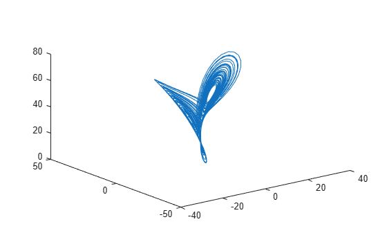
In this example, assume that you have measurements for a Lorenz Attractor. Your measurements are along the x direction only, but the attractor is a three-dimensional system. Using this limited data, reconstruct the phase space such that the properties of the original system are preserved.

Load the Lorenz Attractor data and visualize its x, y and z measurements on a 3-D plot.

load('lorenzAttractorExampleData.mat','data');
plot3(data(:,1),data(:,2),data(:,3));

Estimate the lag and dimension using the x-direction measurement.

xdata = data(:,1);
[~,eLag,eDim] = phaseSpaceReconstruction(xdata)
eLag = 10
eDim = 3

Since the Lorenz Attractor has data in 3 dimensions, the estimated embedding dimension eDim is 3.

Visualize the reconstructed phase space using the estimated lag and embedding dimension.

phaseSpaceReconstruction(xdata,eLag,eDim);

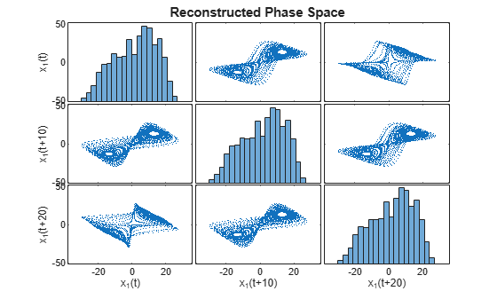
As observed from the 3x3 phase space plot, the topology of the attractor is recovered. x1(t+10) and x1(t+20) are the other two states reconstructed with the estimated lag value of 10. The diagonal plots (1,1), (2,2) and (3,3) represent the histogram of x1(t), x1(t+10)and x1(t+20)data, respectively.

Input Arguments

collapse all

Uniformly sampled time-domain signal, specified as a vector, array, or timetable. When multiple columns exist in X, each column is treated as an independent time series.

If X is specified as a row vector, phaseSpaceReconstruction treats it as a univariate signal.

Embedding dimension, specified as a scalar or vector. dim is the dimension of the space in which you reconstruct a phase portrait starting from your measurements.

When dim is scalar, every column in X is reconstructed using dim. When dim is a vector having same length as the number of columns in X, the reconstruction dimension for column i is dim(i).

Delay value used in phase space reconstruction, specified as a scalar or vector. When lag is scalar, every column in X is reconstructed using lag. When lag is a vector having same length as the number of columns in X, the reconstruction delay for column i is lag(i).

If the time delay is too small, random noise is introduced in the states. In contrast, if the lag is too large, the reconstructed dynamics do not represent the true dynamics of the time series.

Name-Value Arguments

Specify optional pairs of arguments as Name1=Value1,...,NameN=ValueN, where Name is the argument name and Value is the corresponding value. Name-value arguments must appear after other arguments, but the order of the pairs does not matter.

Before R2021a, use commas to separate each name and value, and enclose Name in quotes.

Example: …'HistogramBins',12

Number of bins for discretization, specified as the comma-separated pair consisting of 'HistogramBins' and a scalar. HistogramBins is required to compute the Average Mutual Information (AMI) to estimate delay eLag.

Set the value of HistogramBins based on the length of X.

Maximum value of lag, specified as the comma-separated pair consisting of 'MaxLag' and a scalar. MaxLag is used to estimate delay est_delay using the Average Mutual Information (AMI) algorithm.

Factor to determine embedding dimension, specified as the comma-separated pair consisting of 'PercentFalseNeighbors' and a scalar. When percentage of false nearest neighbors drops below the tuning parameter PercentFalseNeighbors at a dimension d, d is considered as the embedding dimension.

The default value of PercentFalseNeighbors is 0.1 and permissible values lie within the range 0 through 1.

Distance threshold to determine false neighbors, specified as the comma-separated pair consisting of 'DistanceThreshold' and a scalar. DistanceThreshold is a tuning parameter to determine the number of points that are false nearest neighbors in the reconstructed phase space.

The default value of DistanceThreshold is 10, and suggested values lie within the range 10 through 50.

Maximum value of embedding dimension, specified as the comma-separated pair consisting of 'MaxDim' and a scalar.

Change the value of MaxDim if the number of states of your system exceeds 5.

Output Arguments

collapse all

Reconstructed phase space, returned as either an array or timetable. XR contains state vectors based on the embedding dimension and lag value.

Estimated time delay, returned as a scalar, regardless of the size of X.

eLag is estimated using Average Mutual Information (AMI) algorithm. For more information, see Algorithms.

Estimated embedding dimension, returned as a scalar, regardless of the size of X.

eDim is estimated using False Nearest Neighbor (FNN) algorithm. For more information, see Algorithms.

Algorithms

collapse all

Phase Space Reconstruction

For a uniformly sampled univariate time signal X1=(x1,1,x1,2,...,x1,N)T, phaseSpaceReconstruction computes the delayed reconstruction

X1,ir=(x1,i,x1,i+τ1,...,x1,i+(m11)τ1), i=1,2,...,N(m11)τ1

where, N is the length of the time series, τ1 is the lag, and m1 is the embedding dimension for X1.

Similarly, for a multivariate time series X given by,

X=[X1,X2,...,XS]=[x1,1x1,NxS,1xS,N]

phaseSpaceReconstruction computes the reconstruction for each time series as,

Xir=(X1,ir,X2,ir,...,XS,ir), i=1,2,...,N(max{mi}1)(max{τi})

where S is the number of measurements, and N is the length of the time series.

Delay Estimation

The delay for phase space reconstruction is estimated using Average Mutual Information (AMI). For reconstruction, the time delay is set to be the first local minimum of AMI.

Average Mutual Information is computed as,

AMI(T)=i=1Np(xi,xi+T)log2[p(xi,xi+T)p(xi)p(xi+T)]

where, N is the length of the time series and Τ = 1:MaxLag.

Embedding Dimension Estimation

The embedding dimension for phase space reconstruction is estimated using False Nearest Neighbor (FNN) algorithm.

  • For a point i at dimension d, the points Xri and its nearest point Xr*i in the reconstructed phase space {Xri}, i = 1:N, are false neighbors if

    Ri2(d+1)Ri2(d)Ri2(d)>DistanceThreshold

    where, Ri2(d)=XirXir*2 is the distance metric.

  • The estimated embedding dimension d is the smallest value that satisfies the condition pfnn < PercentFalseNeighbors where, pfnn is the ratio of FNN points to total number of points in the reconstructed phase space.

References

[1] Rhodes, Carl & Morari, Manfred. "False Nearest Neighbors Algorithm and Noise Corrupted Time Series." Physical Review. E. 55.10.1103/PhysRevE.55.6162.

[2] Kliková, B., and Aleš Raidl. "Reconstruction of phase space of dynamical systems using method of time delay." Proceedings of the 20th Annual Conference of Doctoral Students WDS 2011.

[3] I. Vlachos, D. Kugiumtzis, "State Space Reconstruction for Multivariate Time Series Prediction", Nonlinear Phenomena in Complex Systems, Vol 11, No 2, pp 241-249, 2008.

[4] Kantz, H., and Schreiber, T. Nonlinear Time Series Analysis. Cambridge: Cambridge University Press, Vol. 7, 2004.

Extended Capabilities

Version History

Introduced in R2018a