Bistatic Clutter Part 2: Visualize and Analyze the Clutter Response

R2026b

Since R2026b

In this example you will learn how to use bistaticClutterSurfaceFIR to rapidly explore how parameter changes (such as pulse repetition interval, position, and velocity) and antenna mounting affect bistatic clutter returns. Instead of running a time-intensive I/Q simulation, you can use automatically generated convenience plots to visualize how system parameters and geometry impact fast-time and slow-time clutter support, clutter range-Doppler map (RDM), overlapping beams and sidelobes on the ground, iso-range and iso-Doppler patterns, and clutter power distribution across the ground. Finally, you will learn how to specify custom pointing for the antenna boresight and visually confirm the results.

This example is part of a three-part series on bistatic clutter. Bistatic Clutter Part 1: Rapidly Generate Clutter Channel FIR and I/Q Radar Data leverages bistaticClutterSurfaceFIR to approximate the clutter channel finite impulse response. Bistatic Clutter Part 3: Simulating Site-Specific Bistatic Land Clutter shows you how to simulate bistatic clutter using bistaticSurfaceReflectivityLand in a radarScenario with GMTED elevation data.

Explore How Parameter Changes Affect Bistatic Clutter Ridge

In this section you will explore how changes in bistatic geometry and relevant parameters affect the clutter ridge.

Define Baseline Simulation Parameters

Set up a baseline bistatic scenario with an X-band transmitter and receiver, mounted on aircraft separated by several kilometers. The transmitter and receiver both use a sinc antenna element with a 10 degree beamwidth in both azimuth and elevation. Positions and velocities are in a flat-earth XYZ frame, where Z=0 is the plane of the surface. In this case, use +Z to be the direction of positive altitude. To simplify, the transmitter and receiver positions and velocity directions are represented by clock-direction terminology.

baselinePRF = 4e3;

alt     = 3e3;
groundR = 10e3;

baselineTxClockPosition = 2;
baselineTxSpeed         = 25;
baselineTxClockVelocity = 5;

baselineTxPose.Position = helperClockPosition(baselineTxClockPosition,groundR,alt);
baselineTxPose.Velocity = helperClockPosition(baselineTxClockVelocity,baselineTxSpeed,0);

baselineRxClockPosition = 11;
baselineRxSpeed         = 25;
baselineRxClockVelocity = 5;

baselineRxPose.Position = helperClockPosition(baselineRxClockPosition,groundR,alt);
baselineRxPose.Velocity = helperClockPosition(baselineRxClockVelocity,baselineRxSpeed,0);

AzBeamwidth   = 10;
ElBeamwidth   = 10;
txAntenna = phased.SincAntennaElement(Beamwidth=[AzBeamwidth ElBeamwidth]);
rxAntenna = phased.SincAntennaElement(Beamwidth=[AzBeamwidth ElBeamwidth]);
swathSize = [40e3 30e3];

Define the radar waveform parameters, including center frequency, pulse repetition frequency (PRF), number of pulses in the CPI, and the sample rate of the system.

sampleRateDesired = 1.5e6;
centerFreq = 10e9;
numPulses = 128;

Call bistaticClutterSurfaceFIR with these baseline values to produce convenience plots. By default, the TransmitterMountingAngles and ReceiverMountingAngles name-value arguments are set to "Auto" (not explicitly listed) so that both antenna boresights point at the swath center like a mechanical spotlight.

baselineSampleRate = round(sampleRateDesired/baselinePRF)*baselinePRF;
bistaticClutterSurfaceFIR(centerFreq,baselineTxPose,baselineRxPose,baselineSampleRate, ...
    TransmitAntenna=txAntenna,ReceiveAntenna=rxAntenna,PRF=baselinePRF,NumPulses=numPulses,SwathSize=swathSize)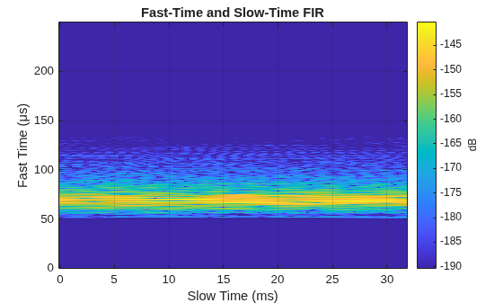

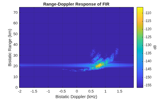
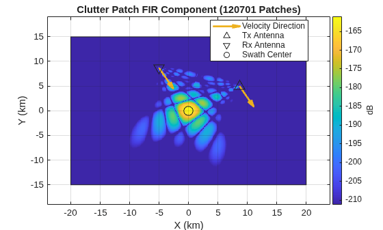
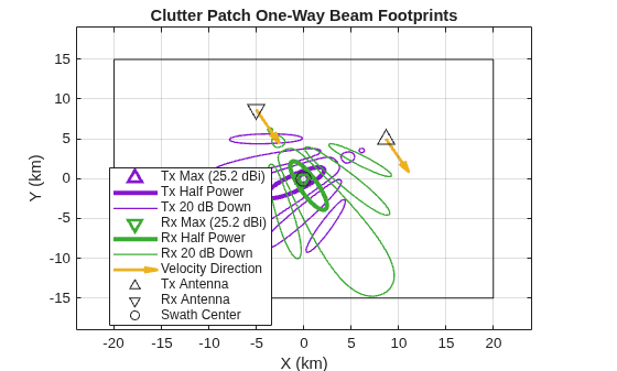
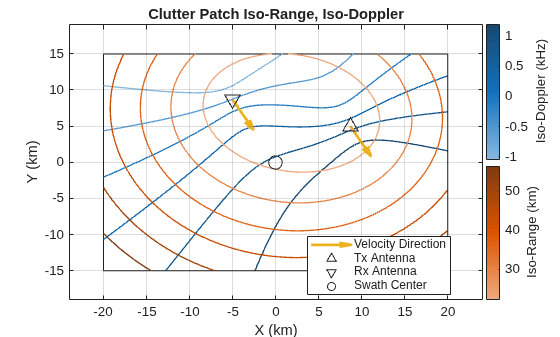
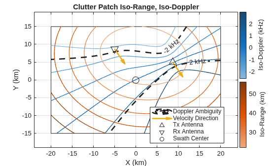
The fast-time and slow-time plot of the FIR shows the clutter returned from surface patches that lie on ellipsoids of constant bistatic range, which correspond to delay bins in fast time. The strongest response in the FIR filter is between 50 and 125 microseconds. The clutter response varies over slow time due to the Doppler shift of individual clutter patches within the ellipsoids. Beyond that region the clutter is below 50 dB from the peak. The range-Doppler projection of the FIR plot shows strong clutter around 20 km bistatic range (total path length from transmitter, to clutter, to receiver) and 750 Hz. The clutter patch FIR component map shows how clutter gain is distributed over the ground. This plot shows strong clutter in the region where the main beams of the transmitter and receiver overlap at the swath center, as well as in the region between the direct path and the swath center, where strong reflectivity and short bistatic range start to overcome the weaker antenna pattern. The beam footprint plot shows the transmit and receive beam patterns on the ground with contour lines, as well as indicators of the location of the clutter patch with maximum gain in the region. The thick colored lines are the antenna half-power beamwidth. The thin lines are 20 dB down from the maximum directivity, which helps indicate both the fuller width of the main lobe and locations of near-in azimuth and elevation sidelobes. This baseline example takes advantage of the default "Auto" antenna pointing behavior to keep both antenna boresights aimed at the swath center like a mechanical spotlight. With this default pointing, you can expect the swath center and maximum gain values to lie on top of each other and the maximum gain to be equivalent to the maximum directivity of each antenna (to within quantization limits of the clutter grid). Finally, the iso-range and iso-Doppler plot shows lines of constant bistatic range and constant bistatic Doppler. The orange lines of bistatic range appear as ellipsoids, while the blue Doppler lines form a more complex structure especially at close ranges. More about these plots can be found in Convenience Plots.

PRF Changes

Explore how changes to PRF affect the clutter plots. Change the PRF to 10 kHz and recompute a round sample rate. Call bistaticClutterSurfaceFIR with no outputs to generate five convenience plots. This increase in PRF will force some clutter in the swath to be range ambiguous.

prf = 10e3;
sampleRate = round(sampleRateDesired/prf)*prf;
bistaticClutterSurfaceFIR(centerFreq,baselineTxPose,baselineRxPose,sampleRate, ...
    TransmitAntenna=txAntenna,ReceiveAntenna=rxAntenna,PRF=prf,NumPulses=numPulses,SwathSize=swathSize)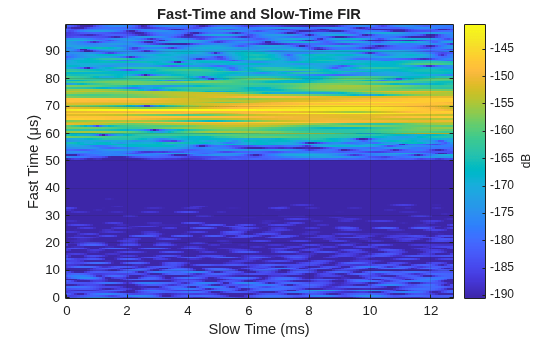

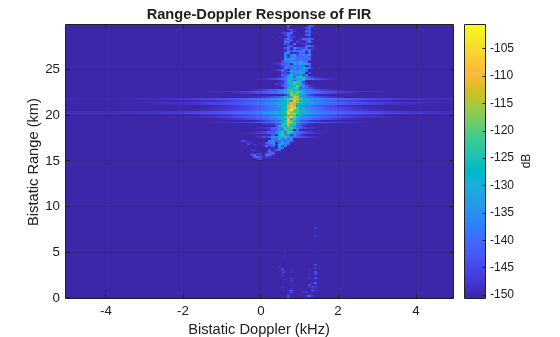
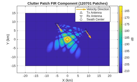
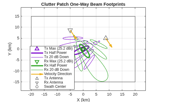
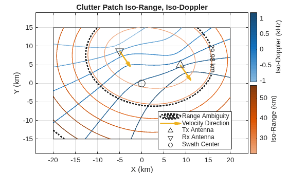
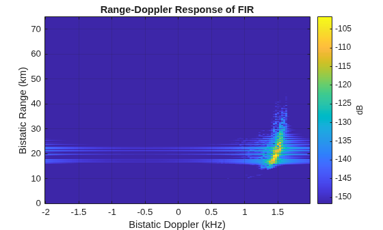
Here we force range ambiguities in the swath. In the fast-time and slow-time plot of the FIR, the strongest clutter still appears around 70 microseconds but notice that the clutter from longer ranges has wrapped into early delays. In fact, the direct path distance is 14 km, corresponding to a delay of 47 microseconds. Clutter and echoes earlier than this are ambiguous. In the range-Doppler projection of the FIR, note how the centroid is still at the same range delay of 20 km, but the plot is now limited to the maximum unambiguous range, around 30 km, and the clutter wraps to close range. The centroid is at the same Doppler, around 0.75 kHz, but the Doppler limits now extend to +/- 5 kHz. With the same number of pulses, you have effectively made your Doppler resolution more coarse. The clutter patch FIR component map and the beam footprint plots are unaffected by changes to the PRF. Finally, look at the iso-range and iso-Doppler plot and note the presence of a thick range ambiguity line at around 30 km. While the iso-range and iso-Doppler colored contour lines do not change with PRF because they are the true range and Doppler, the ambiguity line indicates where the clutter will start to fold over. By comparing this plot to the beam footprints plot, you can see that the main beams are all within the first range ambiguity. If you change the PRF to a small value, you can explore Doppler ambiguities in the clutter.

Position Changes

In this section, you will return to the baseline PRF and sample rate and investigate how moving the transmitter and receiver positions affect the clutter structure.

Smaller Bistatic Angle (12 o'clock and 11 o'clock)

Reset to the baseline poses and move the transmitter to 12 o'clock.

txPose = baselineTxPose;

TxClockPosition = 12;

txPose.Position = helperClockPosition(TxClockPosition,groundR,alt);

bistaticClutterSurfaceFIR(centerFreq,txPose,baselineRxPose,baselineSampleRate, ...
    TransmitAntenna=txAntenna,ReceiveAntenna=rxAntenna,PRF=baselinePRF,NumPulses=numPulses,SwathSize=swathSize)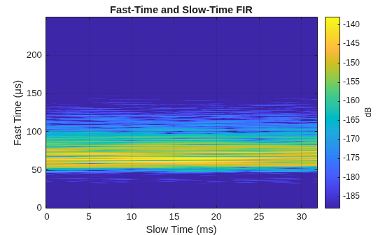

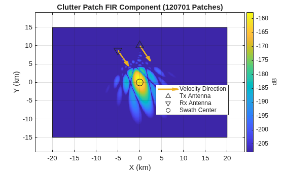
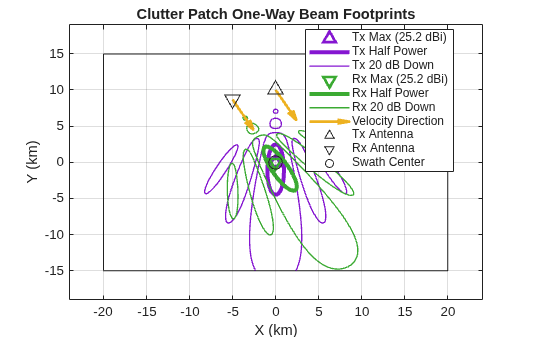
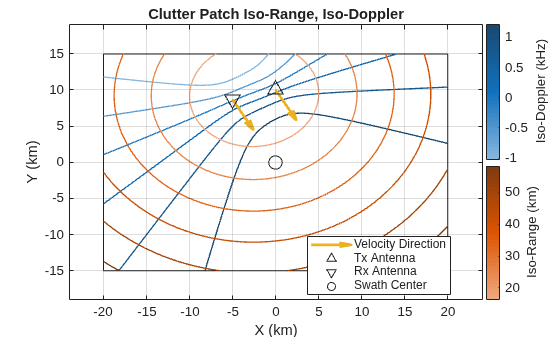
Compared to the baseline plots in Define Baseline Simulation Parameters, the fast-time and slow-time plot of the FIR shows clutter is visible at earlier and later delays as the main beams now have a larger region of overlap. There are fewer sidelobe structures and reduced Doppler spreading in the range-Doppler map. The clutter patch component map indicates little power below the direct path line and mostly mimics the overlapping beam patterns shown in the beam footprints plot. The iso-range and iso-Doppler plot shows that the range ellipsoids have less eccentricity.

Monostatic Configuration (11 o'clock and 11 o'clock)

Continue moving the transmitter until the transmitter and receiver are co-located in a monostatic configuration. Reset the transmitter pose to the baseline parameters and adjust the position so the two sensors are aligned at 11 o'clock.

txPose = baselineTxPose;

TxClockPosition = 11;

txPose.Position = helperClockPosition(TxClockPosition,groundR,alt);

bistaticClutterSurfaceFIR(centerFreq,txPose,baselineRxPose,baselineSampleRate, ...
    TransmitAntenna=txAntenna,ReceiveAntenna=rxAntenna,PRF=baselinePRF,NumPulses=numPulses,SwathSize=swathSize)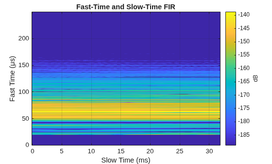

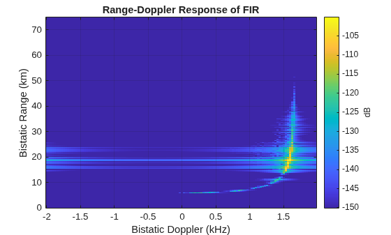
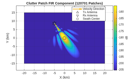
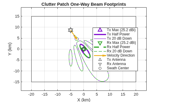
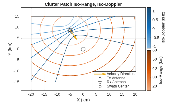
For this monostatic configuration, the fast-time and slow-time plot of the FIR shows clutter at earlier and later delays because the main beams overlap. The range-Doppler map shows far less Doppler spread around the central clutter ridge. Look at the clutter patch FIR component map and beam footprint plot to see the simplified pattern of power and antenna gain on the ground. The iso-range and iso-Doppler plot reduces to the spherical range and symmetric Doppler lines expected from a monostatic system.

Velocity Changes

In this section, you will return to the baseline positions and investigate how changing the transmitter velocity speed and direction affect the clutter structure.

Faster Speed on the Transmit Platform, Maintain Direction (100 m/s)

Reset to the baseline poses and change the transmitter speed to 100 m/s.

txPose = baselineTxPose;
txSpeed = 100;

txPose.Velocity = helperClockPosition(baselineTxClockVelocity,txSpeed,0);

bistaticClutterSurfaceFIR(centerFreq,txPose,baselineRxPose,baselineSampleRate, ...
    TransmitAntenna=txAntenna,ReceiveAntenna=rxAntenna,PRF=baselinePRF,NumPulses=numPulses,SwathSize=swathSize)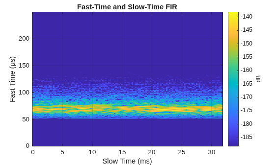

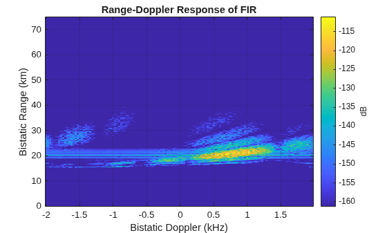
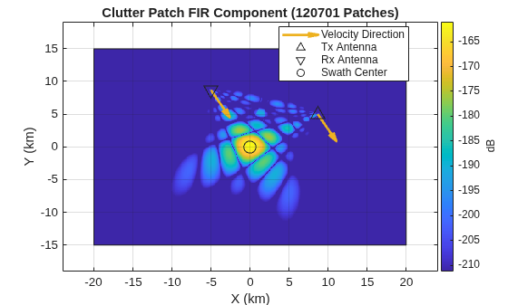
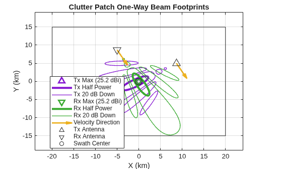
Compared to the baseline plots in Define Baseline Simulation Parameters, the fast-time and slow-time plots of the FIR look similar, but the slow time variation has changed. The range-Doppler projection of the FIR shows this most clearly, as the Doppler spread of the clutter stretches the entire horizontal span, with Doppler wrapping of the clutter from left to right. The clutter patch FIR component map and beam footprints plot are unchanged. The thick Doppler ambiguity line is evident in the iso-range and iso-Doppler plot. Taken together, these plots show that intersections between the receiver main lobe and the transmitter azimuth sidelobes are the primary structures that wrap across the Doppler ambiguity in the range-Doppler map.

Baseline Speed, Change Direction (25 m/s, 11 o'clock)

Reset to the baseline poses and change the transmitter velocity direction to 11 o'clock.

txPose = baselineTxPose;
txClockVelocity = 11;

txPose.Velocity = helperClockPosition(txClockVelocity,baselineTxSpeed,0);

bistaticClutterSurfaceFIR(centerFreq,txPose,baselineRxPose,baselineSampleRate, ...
    TransmitAntenna=txAntenna,ReceiveAntenna=rxAntenna,PRF=baselinePRF,NumPulses=numPulses,SwathSize=swathSize)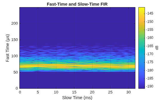

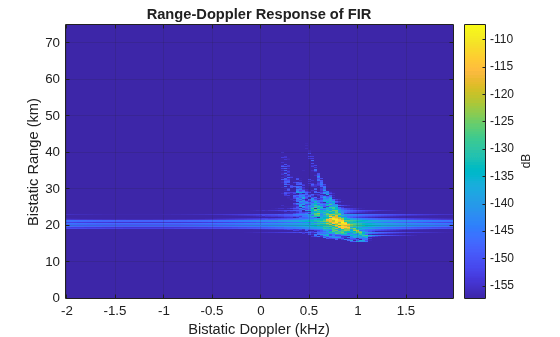
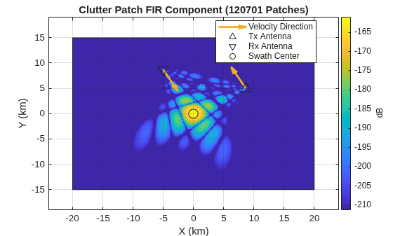
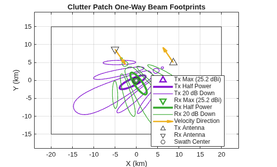
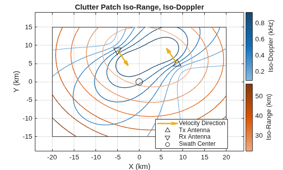
The most notable change resulting from this configuration is evident in the iso-range and iso-Doppler plot. You can see the iso-Doppler lines warp across the swatch. Combined with the beam footprints plot, this shows how the receiver in the upper-left corner observes the same range and Doppler bins across a wide range of angles.

Explore Custom Antenna Pointing

By default, bistaticClutterSurfaceFIR automatically steers the antenna boresights toward the swath center (TransmitterMountingAngles and ReceiverMountingAngles are set to the default value of "Auto"), regardless of the platform orientation specified in txPose. In this section, you will learn how to set custom platform orientation and antenna mounting angles to precisely control where the antenna beams aim in the scene.

Manually point the transmit antenna slightly away from the swath center. Rotate the transmit platform relative to the global XYZ coordinate frame by setting the platform yaw to -60° so the platform's local +X direction aligns with the baseline velocity. Setting the transmitter mounting yaw to -90° would rotate the antenna boresight back toward the swath center. To illustrate custom pointing, set the mounting yaw to -80° instead to demonstrate a 10 degree rotation below the swath center. Finally, set the mounting pitch to the arctangent of the altitude divided by the ground range to tilt the antenna down toward the surface.

PlatformYaw = -60;
txPose = baselineTxPose;
txPose.Orientation = quaternion([PlatformYaw 0 0],'eulerd','ZYX','frame');

MountYaw = -80;
MountPitch = atand(alt/groundR);
txMountingAngles = [MountYaw MountPitch 0];

bistaticClutterSurfaceFIR(centerFreq,txPose,baselineRxPose,baselineSampleRate, ...
    TransmitAntenna=txAntenna,ReceiveAntenna=rxAntenna,PRF=baselinePRF,NumPulses=numPulses, ...
    SwathSize=swathSize,TransmitterMountingAngles=txMountingAngles);

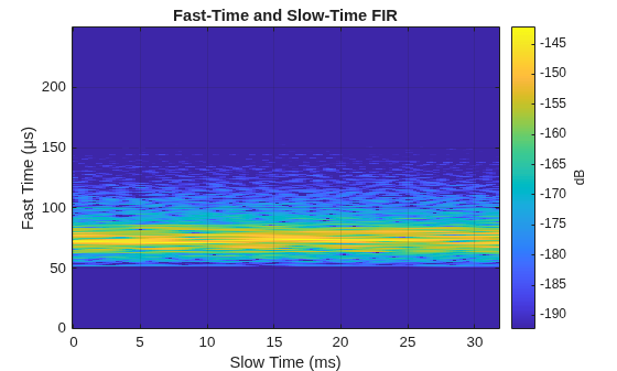
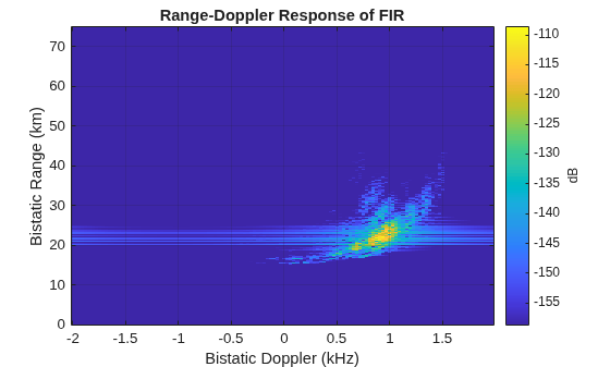
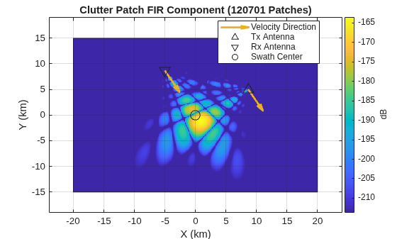
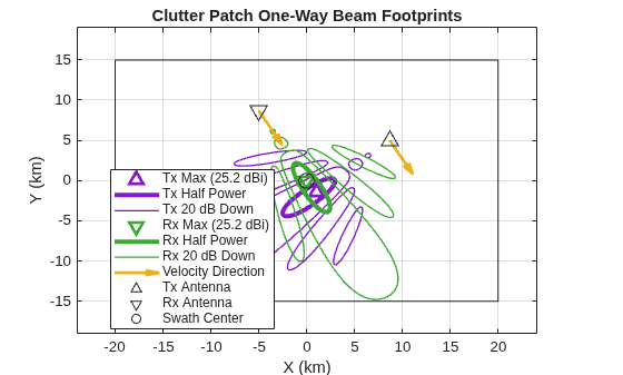
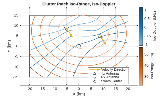
This custom pointing produces plots that are largely similar to the clutter structure shown in the Define Baseline Simulation Parameters section that relies on the default "Auto" pointing behavior. The 10 degree transmitter pointing offset is most evident in the clutter patch FIR component map, which shows the strongest clutter response slightly below the swath center. The platform orientation and antenna mounting angle rotations can be composed and simulated with bistaticClutterSurfaceFIR, similar to other Radar Toolbox™ features such as bistaticFreeSpacePath. For more information, see Radar Coordinate Systems and Frames.

Summary

This example leverages bistaticClutterSurfaceFIR to generate convenience plots and explores how changes to PRF, position, and velocity parameters affect the bistatic clutter structure and spread in the range-Doppler map. You also learned how to steer the antenna boresight using custom platform orientation and sensor mounting angles.

References

1. Willis, Nicholas J., and Hugh D. Griffiths, eds. "Advances in bistatic radar." Vol. 2. SciTech Publishing, 2007.

2. Maitland, C., D. Mountford, B. Hopson, A. Glass, J. Patel, E. Rose, P. Durham, and P. McGinley. "Development of a Bistatic Clutter Tool and Validation by Experimental Data." IET Conference Proceedings 2022, no. 17 (March 2, 2023): 125–29.

Helper Functions

function pos = helperClockPosition(hour, groundDistance, altitude)
az = hour * 30;
pos = [groundDistance * sind(az), groundDistance * cosd(az), altitude];
end