Train and Deploy a YOLOX Object Detector on Raspberry Pi Using Transfer Learning

R2026b

This example shows how to create a custom object detection application for Raspberry Pi® using YOLOX and transfer learning. The workflow guides you through labeling custom training data, training and evaluating a YOLOX-nano detector, packaging the trained model for deployment, and deploying the application to Raspberry Pi using Simulink®. The deployed application performs real-time object detection on live camera input.

Using this example, you learn how to:

Label custom objects in video data using the Video Labeler (Computer Vision Toolbox).
Train a YOLOX-nano object detector using transfer learning.
Evaluate detection performance on a validation set.
Deploy the trained model to Raspberry Pi using Simulink and run real-time object detection.

Hardware Requirements

Raspberry Pi 5 (recommended, 4 GB or 8 GB RAM) or Raspberry Pi 4B (4 GB or 8 GB RAM)
Raspberry Pi Camera Module V2 or V3
5V power supply (5A for Pi 5, 3A for Pi 4B)
MicroSD card (16 GB+, Class 10)
Ethernet cable or WiFi connection (between Raspberry Pi and host computer)

Note: For best inference performance, use Raspberry Pi 5. Raspberry Pi 4 Model B is also supported but provides lower frame rates during real-time object detection.

Set Up Project Structure

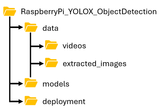
Before collecting data or training a model, create a dedicated project folder with subfolders to organize training data, trained models, and deployment artifacts. Using a consistent folder structure helps you manage datasets, model files, and deployment packages throughout the workflow.

The folder layout maps directly to the workflow:

videos — Store source video files here before labeling.
extracted_images — Store images extracted from labeled data.
models — Save trained YOLOX detector models.
deployment — Save deployment packages used by model.

%% Set Up Project Structure
% Create folders for training data, models, and deployment files.

PROJECT_NAME = 'RaspberryPi_YOLOX_ObjectDetection'; % Root project folder name
DATA_FOLDER = fullfile(PROJECT_NAME, 'data'); % Parent folder for all data files
VIDEO_FOLDER = fullfile(DATA_FOLDER, 'videos'); % Store raw video recordings here
IMAGES_FOLDER = fullfile(DATA_FOLDER, 'extracted_images'); % Extracted frames written here during labeling
MODELS_FOLDER = fullfile(PROJECT_NAME, 'models'); % Trained detector saved here
DEPLOYMENT_FOLDER = fullfile(PROJECT_NAME, 'deployment'); % Deployment package for Raspberry Pi

% Create directories if they don't exist
folders = {DATA_FOLDER, VIDEO_FOLDER, IMAGES_FOLDER, MODELS_FOLDER, DEPLOYMENT_FOLDER};

for i = 1:length(folders)
    if ~exist(folders{i}, 'dir')
        mkdir(folders{i});
    end
end

Collect and Label Training Data

Record a short video (30-60 seconds) of your target object from multiple angles and lighting conditions. Place the video file in the videos folder created in the previous step. For transfer learning with YOLOX, aim for approximately 500 to 900 images per class.

videoLabeler;

Launch the app and click Import > From File and select the pre-recorded video from the videos folder.
In the left panel, under ROI Labels, click + and create a rectangular label for each object class.
Draw bounding boxes on 10–20 frames manually.
Click Automate and select Point Tracker to propagate labels across remaining frames.
Review tracked labels and correct any tracking drift.
Click Export Labels > To Workspace and name the variable gTruth.

Save the exported labels for use during training.

if exist('gTruth', 'var') % Check if gTruth was exported from Video Labeler
    GROUND_TRUTH_FILE = fullfile(DATA_FOLDER, 'gTruth.mat'); % Define save path for labeled data
    save(GROUND_TRUTH_FILE, 'gTruth'); % Save ground truth to .mat file for training
    fprintf('✓ Ground truth saved: %s\n', GROUND_TRUTH_FILE);

    % Display summary
    fprintf('\nDataset Summary:\n');
    fprintf('  Total frames: %d\n', height(gTruth.DataSource));
    fprintf('  Label definitions: %d\n', height(gTruth.LabelDefinitions));
    fprintf('  Classes: %s\n', strjoin(gTruth.LabelDefinitions.Name, ', '));
else
    warning('gTruth variable not found. Please export from Video Labeler first.');
end

Warning: gTruth variable not found. Please export from Video Labeler first.

Verify Labeled Data

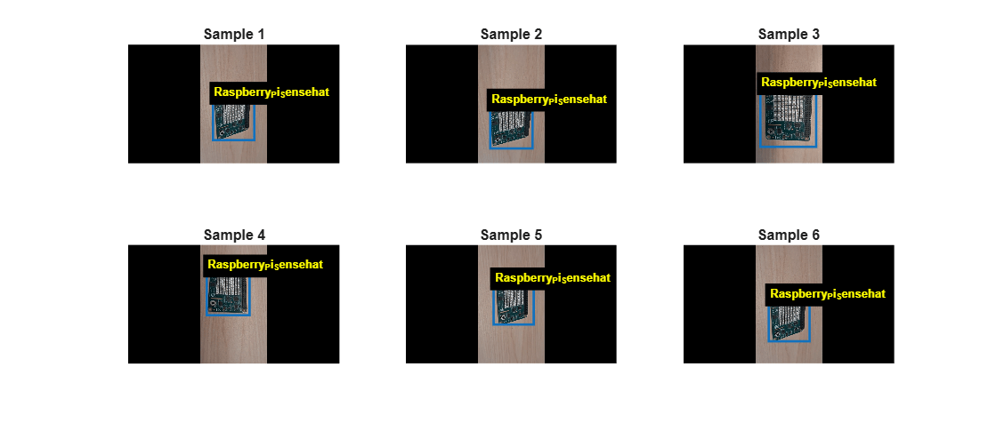
Before training, inspect the labeled data to confirm that bounding boxes are accurate and that you have enough annotated frames for each class. Inspect annotation statistics and visualize sample images to confirm that bounding boxes align correctly with the target objects. Review the visualized samples to check that boxes fit your objects and that no labels are missing or misplaced.

Load Ground Truth Data

Load the ground truth data exported from the Video Labeler (Computer Vision Toolbox) and convert it into a training dataset.

% Load and verify ground truth data
GROUND_TRUTH_FILE = fullfile(DATA_FOLDER, 'gTruth.mat');

if isfile(GROUND_TRUTH_FILE)
    load(GROUND_TRUTH_FILE, 'gTruth');
    
    % Extract training data
    trainingData = objectDetectorTrainingData(gTruth, ...
        'SamplingFactor', 1, ...
        'WriteLocation', IMAGES_FOLDER);
    
    % Statistics
    numImages = height(trainingData);
    numClasses = width(trainingData) - 1;
    
    fprintf('✓ Dataset loaded successfully\n');
    fprintf('  Total samples: %d\n', numImages);
    fprintf('  Number of classes: %d\n', numClasses);
    
    % Minimum dataset check
    MIN_RECOMMENDED = 500;
    if numImages < MIN_RECOMMENDED
        fprintf('\n️ WARNING: You have %d images. Recommended: %d+ images per class\n', ...
                numImages, MIN_RECOMMENDED);
        fprintf('   Consider capturing more video footage for better results.\n\n');
    else
        fprintf('  ✓ Dataset size is good for transfer learning!\n\n');
    end

Write images extracted to folder: 
    RaspberryPi_YOLOX_ObjectDetection\data\extracted_images
Writing images extracted from Sample_Video.mp4: 0/515
Completed.

✓ Dataset loaded successfully

  Total samples: 515

  Number of classes: 1

  ✓ Dataset size is good for transfer learning!

Review Dataset Statistics

Review the number of images and annotations for each object class.

% Count boxes per class
classNames = trainingData.Properties.VariableNames(2:end);
fprintf('  Boxes per class:\n');

  Boxes per class:

for i = 1:numClasses
        className = classNames{i};
        classData = trainingData.(className);
        totalBoxes = sum(cellfun(@(x) size(x, 1), classData));
        framesWithClass = sum(cellfun(@(x) ~isempty(x), classData));
        fprintf('    %s: %d boxes across %d frames\n', ...
                className, totalBoxes, framesWithClass);

    Raspberry_Pi_Sensehat: 515 boxes across 515 frames

end

Visualize Sample Annotations

Display a random subset of labeled images to verify annotation quality.

% Visualize random samples
    figure('Name', 'Labeled Data Samples', 'Position', [100, 100, 1400, 600]);
    numSamples = min(6, numImages); % Show up to 6 samples
    indices = randperm(numImages, numSamples); % Select random frames
    
    for i = 1:numSamples
        subplot(2, 3, i);

        idx = indices(i);
        img = imread(trainingData{idx, 1}{1});
        imshow(img);
        hold on;
        
        % Draw all bounding boxes for this image
        colors = lines(numClasses);
        for c = 1:numClasses
            boxes = trainingData{idx, c+1}{1};
            if ~isempty(boxes)
                for b = 1:size(boxes, 1)
                    rectangle('Position', boxes(b, :), ...
                             'EdgeColor', colors(c, :), 'LineWidth', 2);
                    text(boxes(b, 1), boxes(b, 2) - 5, classNames{c}, ...
                         'Color', 'yellow', 'FontWeight', 'bold', ...
                         'BackgroundColor', 'black', 'FontSize', 10);
                end
            end
        end
        hold off;
        title(sprintf('Sample %d', i), 'FontSize', 12);
    end
    
    fprintf('\n✓ Data quality verification complete\n');

✓ Data quality verification complete

    fprintf('  Review the visualization to ensure labels are correct\n\n');

  Review the visualization to ensure labels are correct

    
else
    warning('Ground truth file not found: %s', GROUND_TRUTH_FILE);
    fprintf('Please complete video labeling first.\n\n');
end

Configure YOLOX Training

Train a YOLOX-nano detector using transfer learning on your custom dataset. Select a YOLOX model variant based on your accuracy and performance requirements. Smaller models provide faster inference and lower memory usage, while larger models typically deliver higher detection accuracy at the expense of inference speed. This example uses the YOLOX-nano variant as it provides the best balance of speed, memory footprint, and accuracy for Raspberry Pi deployment.

If your application requires higher accuracy and can tolerate slower inference, switch to tiny-coco and increase inputSize to [640 640 3].

YOLOX Model Selection

This table compares the YOLOX model variants that are suitable for deployment on Raspberry Pi hardware. As the model size increases, the detector typically provides higher accuracy but requires more memory and longer inference times. Use this comparison to select a model that balances accuracy and real-time performance for your application.

The Inference (Pi 5) and Inference (Pi 4B) columns indicate the approximate time required to process a single image. Lower inference times generally result in higher frame rates and more responsive real-time detection.

Model	Size	Inference (Pi 5)	Inference (Pi 4B)	Use Case
nano-coco	~ 3MB	~100-150 ms	~200-300 ms	Best balance of speed and accuracy for Raspberry Pi deployment.
tiny-coco	~ 8MB	~150-250 ms	~300-500 ms	Choose when improved detection accuracy is more important than inference speed.
small-coco	~ 15 MB	~250-400 ms	~500-800 ms	Choose when maximizing detection accuracy is the highest priority.
medium-coco	~40 MB	~400-700ms	~800-1500ms	Suitable for desktop or powerful edge devices.

% Configuration structure
CONFIG = struct();

% Paths
CONFIG.groundTruthFile = GROUND_TRUTH_FILE;
CONFIG.outputFolder = IMAGES_FOLDER;
CONFIG.modelSavePath = fullfile(MODELS_FOLDER, 'trainedYOLOXDetector.mat');

% Data split
CONFIG.trainRatio = 0.85; % 85% train, 15% validation

% YOLOX Model Selection
% Options: 'nano-coco', 'tiny-coco', 'small-coco', 'medium-coco'
CONFIG.modelName = 'nano-coco'; % Recommended for Raspberry Pi

% Input size - affects accuracy and speed
% Larger = better accuracy but slower
% Common sizes: [320, 320], [416, 416], [640, 640]
CONFIG.inputSize = [416, 416, 3]; % Good balance for RPi

% Training hyperparameters (optimized for small datasets)
CONFIG.learningRate = 1e-3;
CONFIG.miniBatchSize = 8;
CONFIG.maxEpochs = 60;
CONFIG.validationFrequency = 10;
CONFIG.verboseFrequency = 5;
CONFIG.executionEnvironment = 'auto'; % auto, cpu, gpu

% Learning rate schedule
CONFIG.learnRateDropFactor = 0.1;
CONFIG.learnRateDropPeriod = 20;

% Data augmentation (helps prevent overfitting)
CONFIG.augmentation.horizontalFlip = true;
CONFIG.augmentation.brightness = 0.15;
CONFIG.augmentation.contrast = 0.15;
CONFIG.augmentation.saturation = 0.1;

Split Data into Training and Validation Sets

Divide the labeled dataset into a training set and a validation set. Use the training dataset to fine-tune the detector and reserve the validation dataset for monitoring training progress and evaluating detector performance. The training set teaches the detector to recognize your objects, while the validation set measures how well the detector generalizes to images it has not seen during training. An 85/15 split retains enough data for effective learning while reserving a representative subset for performance evaluation.

if ~isfile(CONFIG.groundTruthFile)
    error('Ground truth file not found: %s\nPlease complete Part 1 first.', ...
          CONFIG.groundTruthFile);
end

load(CONFIG.groundTruthFile, 'gTruth');

% Extract training data
trainingData = objectDetectorTrainingData(gTruth, ...
    'SamplingFactor', 1, ...
    'WriteLocation', CONFIG.outputFolder);

Write images extracted to folder: 
    RaspberryPi_YOLOX_ObjectDetection\data\extracted_images
Writing images extracted from Sample_Video.mp4: 0/515
Completed.

numSamples = height(trainingData);
classNames = trainingData.Properties.VariableNames(2:end);

% Check minimum requirements
MIN_SAMPLES = 300;
RECOMMENDED_SAMPLES = 500;

if numSamples < MIN_SAMPLES
    error(['Insufficient training data (%d samples).\n' ...
        'Minimum required: %d samples.\n' ...
        'Recommended: %d+ samples per class.\n' ...
        'Please capture and label more video footage.'], ...
        numSamples, MIN_SAMPLES, RECOMMENDED_SAMPLES);
elseif numSamples < RECOMMENDED_SAMPLES
    warning('Dataset has %d samples. Recommended: %d+ for optimal results.', ...
        numSamples, RECOMMENDED_SAMPLES);
    fprintf('  Training will continue, but consider adding more data.\n');
end

% Train/validation split
rng(42); % For reproducibility
idx = randperm(numSamples);
numTrain = round(CONFIG.trainRatio * numSamples);

trainData = trainingData(idx(1:numTrain), :);
valData = trainingData(idx(numTrain+1:end), :);

Create Datastores with Augmentation

Create datastores for the training and validation datasets. Datastores load images and bounding boxes in batches during training instead of loading the entire dataset into memory, which helps manage memory usage for larger datasets.

Apply data augmentation to the training dataset to improve detector robustness and reduce overfitting. During training, the datastore resizes images to match the detector input size and applies random transformations, such as horizontal flipping and color jitter. These augmentations increase data diversity and help the detector generalize to variations in object appearance, lighting conditions, and viewing angles. The validation datastore applies only image resizing so that evaluation reflects detector performance on unmodified data.

% Training datastore with augmentation
dsTrain = createOptimizedDatastore(trainData, CONFIG, true);

% Validation datastore (no augmentation)
dsVal = createOptimizedDatastore(valData, CONFIG, false);

fprintf('✓ Datastores created\n');

✓ Datastores created

Verify the datastore by reading one sample. Confirm that the output image matches the expected input size and that bounding boxes are present.

% Verify datastore by reading one sample
reset(dsTrain);
sample = read(dsTrain);
fprintf('✓ Datastore verification:\n');

✓ Datastore verification:

Create YOLOX Detector

Create a YOLOX object detector initialized with weights pretrained on the COCO dataset (80 object classes, over 100,000 images). Transfer learning reuses these pretrained feature extraction layers and replaces only the final detection head to match your custom classes. This approach reduces training time and requires fewer labeled images than training a detector from scratch.

Configure training options using the Stochastic Gradient Descent with Momentum (SGDM) with a piecewise learning rate schedule. The learning rate drops by a factor of 10 every 20 epochs which helps the detector converge to a stable solution in the later stages of training.

%% Create YOLOX Detector
detector = yoloxObjectDetector(CONFIG.modelName, classNames, ...
    'InputSize', CONFIG.inputSize); % Create detector with pretrained COCO weights

%% Configure Training Options
options = trainingOptions('sgdm', ...
    'InitialLearnRate', CONFIG.learningRate, ...
    'MiniBatchSize', CONFIG.miniBatchSize, ...
    'MaxEpochs', CONFIG.maxEpochs, ...
    'ExecutionEnvironment', CONFIG.executionEnvironment, ...
    'ResetInputNormalization', false, ...
    'Shuffle', 'every-epoch', ...
    'ValidationData', dsVal, ...
    'ValidationFrequency', CONFIG.validationFrequency, ...
    'VerboseFrequency', CONFIG.verboseFrequency, ...
    'Plots', 'training-progress', ...
    'LearnRateSchedule', 'piecewise', ...
    'LearnRateDropFactor', CONFIG.learnRateDropFactor, ...
    'LearnRateDropPeriod', CONFIG.learnRateDropPeriod, ...
    'CheckpointPath', tempdir);

Train YOLOX Detector

Train the detector using transfer learning. During training, a progress plot opens automatically showing the training loss (blue line) and validation loss (orange line). Monitor the training progress to verify that the loss decreases and stabilizes over successive iterations. A widening gap between them indicates overfitting — the model memorizes training data instead of learning generalizable patterns.

Training time depends on the available hardware. Systems with a supported GPU typically complete training faster than CPU-only systems.

% Train YOLOX detector
doTraining = false

doTraining = logical
   0

if doTraining
    reset(dsTrain);
    tic;
    try
        [trainedDetector, trainingInfo] = trainYOLOXObjectDetector(dsTrain, detector, options);
        trainingTime = toc;

        fprintf('\n========================================\n');
        fprintf(' TRAINING COMPLETED SUCCESSFULLY!\n');
        fprintf('========================================\n');
        fprintf('  Total time: %.1f minutes (%.0f seconds)\n', trainingTime/60, trainingTime);
        fprintf('  Final training loss: %.4f\n', trainingInfo(end,1).TrainingYoloXLoss);

        if isfield(trainingInfo, 'ValidationYoloXLoss') && ~isempty(trainingInfo(end).ValidationYoloXLoss)
            fprintf('  Final validation loss: %.4f\n', trainingInfo(end,1).ValidationYoloXLoss);
        end

        fprintf('========================================\n\n');

        % Save the trained model
        detector = trainedDetector;
        save(CONFIG.modelSavePath, 'detector');
        fprintf('✓ Model saved: %s\n\n', CONFIG.modelSavePath);

    catch ME
        fprintf('\n TRAINING FAILED\n');
        fprintf('Error: %s\n\n', ME.message);
        fprintf('Stack trace:\n');
        disp(getReport(ME, 'extended'));
        fprintf('\nPlease check the Troubleshooting section below.\n\n');
        rethrow(ME);
    end
else
    load(CONFIG.modelSavePath, 'detector');
end

Evaluate Trained Detector

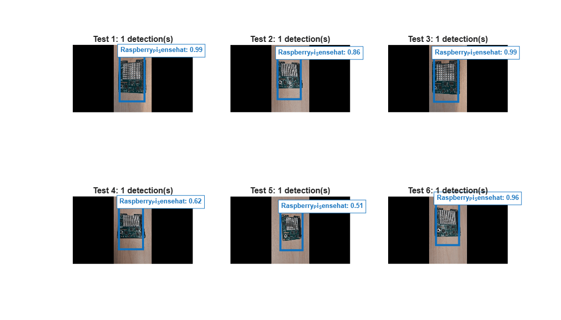
Evaluate the trained detector on validation images before deploying it to Raspberry Pi hardware. This step confirms that the detector generalizes to images it has never seen. Examine the confidence scores alongside each detection — scores above 0.7 indicate strong recognition, scores between 0.5 and 0.7 indicate moderate confidence, and scores below 0.5 suggest the detector needs more training data or additional epochs.

Run the detector on a subset of validation images and visualize the predicted bounding boxes, labels, and confidence scores. If detections are missing or confidence is low, revisit the labeling quality in the verification step or increase maxEpochs and retrain.

%% Evaluate Trained Detector
numTestSamples = min(6, height(valData)); % Evaluate up to 6 validation images
testIndices = randperm(height(valData), numTestSamples); % Select random validation samples

avgConfidence = 0;
avgDetections = 0;
validDetectionCount = 0;

figure('Name', 'YOLOX Detection Results on Validation Set', ...
       'Position', [100, 100, 1400, 800]);

for i = 1:numTestSamples
    idx = testIndices(i);
    testImg = imread(valData{idx, 1}{1});
    
    % Detect objects
    [bboxes, scores, labels] = detect(detector, testImg, 'Threshold', 0.3);
    
    % Calculate statistics
    if ~isempty(bboxes)
        avgConfidence = avgConfidence + mean(scores);
        avgDetections = avgDetections + size(bboxes, 1);
        validDetectionCount = validDetectionCount + 1;
    end
    
    % Visualize
    subplot(2, 3, i);
    imshow(testImg);
    hold on;
    
    if ~isempty(bboxes)
        colors = lines(length(classNames));
        for j = 1:size(bboxes, 1)
            % Get color based on class
            classIdx = find(strcmp(classNames, char(labels(j))));
            if isempty(classIdx)
                classIdx = 1;
            end
            color = colors(classIdx, :);
            
            % Draw box
            rectangle('Position', bboxes(j, :), ...
                     'EdgeColor', color, 'LineWidth', 3);
            
            % Add label with confidence
            label = sprintf('%s: %.2f', char(labels(j)), scores(j));
            text(bboxes(j, 1), bboxes(j, 2) - 10, label, ...
                'Color', color, 'FontSize', 10, 'FontWeight', 'bold', ...
                'BackgroundColor', 'white', 'EdgeColor', color);
        end
    end
    
    hold off;
    title(sprintf('Test %d: %d detection(s)', i, size(bboxes, 1)), ...
          'FontSize', 12, 'FontWeight', 'bold');
end

Detection Summary

Compute a simple summary of detector performance on the validation samples.

%% Detection summary
if validDetectionCount > 0
    avgConfidence = avgConfidence / validDetectionCount;
    avgDetections = avgDetections / numTestSamples;
else
    avgConfidence = 0;
    avgDetections = 0;
end

% Interpret results
if avgConfidence > 0.7
    fprintf('  Excellent detection confidence!\n');
elseif avgConfidence > 0.5
    fprintf('  Good detection confidence.\n');
elseif avgConfidence > 0.3
    fprintf('  Moderate confidence. Consider more training data.\n');
else
    fprintf('  Low confidence. Review training data quality.\n');
end

  Excellent detection confidence!

Visualize Training Metrics

Review the training and validation loss curves to assess convergence and identify potential overfitting. Plot the training and validation loss curves to assess how well the detector learned over time. A healthy training run shows both curves decreasing and leveling off.

Typical training outcomes include:

Training and validation loss decrease and stabilize indicating that the detector has learned useful features from the dataset.
Training loss decreases while validation loss increases, indicating overfitting. Reduce maxEpochs or increase dataset diversity.
Training and validation loss do not decrease substantially, indicating that the learning rate may be too low or that the training data requires further review.

if doTraining
figure('Name', 'Training Metrics', 'Position', [100, 100, 1200, 500]);

% Extract training loss values from struct array
trainingLoss = [trainingInfo.TrainingYoloXLoss];

% Plot training loss
subplot(1, 2, 1);
plot(trainingLoss, 'LineWidth', 2, 'Color', [0 0.4470 0.7410]);
xlabel('Iteration', 'FontSize', 12, 'FontWeight', 'bold');
ylabel('Training Loss', 'FontSize', 12, 'FontWeight', 'bold');
title('Training Loss Over Time', 'FontSize', 14, 'FontWeight', 'bold');
grid on;
xlim([1, length(trainingInfo)]);

% Add annotations
minLoss = min(trainingLoss);
[~, minIdx] = min(trainingLoss);
hold on;
plot(minIdx, minLoss, 'r*', 'MarkerSize', 15, 'LineWidth', 2);
text(minIdx, minLoss, sprintf('  Min: %.4f', minLoss), ...
     'FontSize', 10, 'FontWeight', 'bold', 'Color', 'red');
hold off;

% Plot validation loss if available
subplot(1, 2, 2);
if isfield(trainingInfo, 'ValidationYoloXLoss')
    validationLoss = [trainingInfo.ValidationYoloXLoss];
    % Remove NaN or empty values
    validIdx = ~isnan(validationLoss);
    
    if any(validIdx)
        plot(find(validIdx), validationLoss(validIdx), 'LineWidth', 2, 'Color', [0.8500 0.3250 0.0980]);
        xlabel('Validation Iteration', 'FontSize', 12, 'FontWeight', 'bold');
        ylabel('Validation Loss', 'FontSize', 12, 'FontWeight', 'bold');
        title('Validation Loss Over Time', 'FontSize', 14, 'FontWeight', 'bold');
        grid on;
        
        % Check for overfitting
        validValLoss = validationLoss(validIdx);
        if length(validValLoss) > 5
            recentValLoss = validValLoss(end-4:end);
            if all(diff(recentValLoss) > 0)
                text(0.5, 0.5, 'Warning: Validation loss increasing (possible overfitting)', ...
                     'Units', 'normalized', 'HorizontalAlignment', 'center', ...
                     'FontSize', 10, 'Color', 'red', 'FontWeight', 'bold');
            end
        end
    else
        text(0.5, 0.5, 'Validation loss not recorded', ...
             'Units', 'normalized', 'HorizontalAlignment', 'center', ...
             'FontSize', 12);
    end
else
    text(0.5, 0.5, 'Validation loss not recorded', ...
         'Units', 'normalized', 'HorizontalAlignment', 'center', ...
         'FontSize', 12);
end
else
    fprintf("To train the detector, set doTraining to true and rerun this section. trainingInfo is created only when trainYOLOXObjectDetector runs to completion. If you skipped training, this variable does not exist in the workspace and its fields TrainingYoloXLoss and ValidationYoloXLoss are not available.");
end

To train the detector, set doTraining to true and rerun this section. trainingInfo is created only when trainYOLOXObjectDetector runs to completion. If you skipped training, this variable does not exist in the workspace and its fields TrainingYoloXLoss and ValidationYoloXLoss are not available.

Prepare Deployment Package

Package the trained detector and model configuration for deployment to Raspberry Pi. The deployment package stores the trained YOLOX detector, class names, and detector configuration in a MAT-file that the model loads during deployment.

Separating the deployment package from the training artifacts allows you to retrain the model and redeploy without modifying the model — just regenerate this package and rebuild.

% Define deployment configuration from CONFIG
deployConfig.functionName = 'deploy_yolox_realtime';
deployConfig.detectorFile = CONFIG.modelSavePath;
deployConfig.inputSize = CONFIG.inputSize;
deployConfig.detectionThreshold = 0.3;
deployConfig.cameraResolution = '640x480';
deployConfig.cameraIndex = 1;

% Generate the deployment function
functionCode = sprintf(['function %s()\n' ...
    '%% YOLOX Real-Time Object Detection for Raspberry Pi\n' ...
    '%% \n' ...
    '%% Usage:\n' ...
    '%%   Run in MATLAB: %s() - Runs on host, captures from RPi camera\n' ...
    '%% \n' ...
    '%% Deployment to Raspberry Pi:\n' ...
    '%%   board = targetHardware(''Raspberry Pi (64bit)'');\n' ...
    '%%   deploy(board, ''%s.m'');\n\n' ...
    '%% 1. Load the fine-tuned detector\n' ...
    'persistent fineTunedDetector;\n' ...
    'if isempty(fineTunedDetector)\n' ...
    '    fineTunedDetector = coder.loadDeepLearningNetwork(''%s'');\n' ...
    'end\n\n' ...
    '%% 2. Create a connection to the Raspberry Pi hardware\n' ...
    'r = raspi();\n\n' ...
    '%% 3. Connect to Raspberry Pi camera\n' ...
    'cam = webcam(r, %d, ''%s'');\n\n' ...
    '%% 4. Real-time detection loop\n' ...
    'while true\n' ...
    '    img = snapshot(cam);\n' ...
    '    img = imresize(img, [%d %d]);\n' ...
    '    \n' ...
    '    [bboxes, scores, labels] = detect(fineTunedDetector, img, ...\n' ...
    '                                      ''Threshold'', %.2f);\n' ...
    '    \n' ...
    '    if ~isempty(bboxes)\n' ...
    '        img = insertObjectAnnotation(img, ''rectangle'', bboxes, labels);\n' ...
    '    end\n' ...
    '    \n' ...
    '    displayImage(r, img, ''Title'', ''YOLOX Object Detection'');\n' ...
    'end\n\n' ...
    'end\n'], ...
    deployConfig.functionName, ...
    deployConfig.functionName, ...
    deployConfig.functionName, ...
    deployConfig.detectorFile, ...
    deployConfig.cameraIndex, ...
    deployConfig.cameraResolution, ...
    deployConfig.inputSize(1), deployConfig.inputSize(2), ...
    deployConfig.detectionThreshold);

% Save the deployment function
deploymentFile = sprintf('%s.m', deployConfig.functionName);
fid = fopen(deploymentFile, 'w');
fprintf(fid, '%s', functionCode);
fclose(fid);

fprintf('✓ Deployment function generated: %s\n\n', deploymentFile);

✓ Deployment function generated: deploy_yolox_realtime.m

Deploy Trained Detector Using MATLAB

Review the generated code and change settings like webcam index and Raspberry Pi hostname, and then follow these steps.

1. Test image on host using Raspberry Pi camera — Open the generated deployment function in the MATLAB Editor and click Run in the Editor tab under the Run section. This runs the trained YOLOX detector on your development computer while capturing live frames from the Raspberry Pi camera, verifying that the detector works correctly before deploying standalone code to the hardware.

verifyOnHost = false

verifyOnHost = logical
   0

if verifyOnHost
    deploy_yolox_realtime();
else
    fprintf("To verify detection on the host, set verifyOnHost to true and rerun this section.\nMake sure you have previously connected to your Raspberry Pi using raspi('hostname','username','password') and that a webcam is attached to the board.\n");
end

To verify detection on the host, set verifyOnHost to true and rerun this section.
Make sure you have previously connected to your Raspberry Pi using raspi('hostname','username','password') and that a webcam is attached to the board.

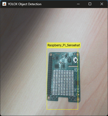
2. Deploy to Raspberry Pi — Deploy the detector as a standalone application on the Raspberry Pi hardware. Run the following commands in the MATLAB Command Window to generate C code from the deployment function, cross-compile it for the Raspberry Pi, and start execution on the board. Once deployed, the application runs independently without requiring a MATLAB connection.

doDeployment = false

doDeployment = logical
   0

if doDeployment
    board = targetHardware('Raspberry Pi (64bit)');
    deploy(board,'deploy_yolox_realtime');
else
    fprintf("To deploy to Raspberry Pi, set doDeployment to true and rerun this section.\n");
end

To deploy to Raspberry Pi, set doDeployment to true and rerun this section.

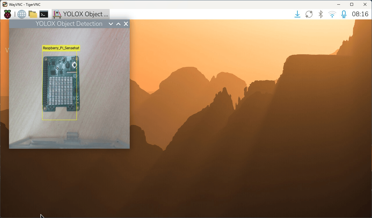
Deploy Trained Detector Using Simulink

To deploy the trained YOLOX detector as a standalone application, use the pre-configured model (raspberrypi_custom_object_detection.slx). The model integrates camera capture, preprocessing, inference, and display into a single deployable system that runs independently on Raspberry Pi without requiring a MATLAB connection.

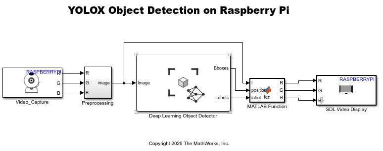
open_system('raspberrypi_custom_object_detection.slx');

The model loads the deployment package created in the previous section and uses it during code generation and deployment.

The model contains the following key components:

Raspberry Pi Camera Video Capture — Acquires RGB frames from the Raspberry Pi camera.
Preprocessing subsystem — Concatenates the R, G, B channels into a single image and resizes it to match the detector input size (416x416).
Deep Learning Object Detector block — Runs the trained YOLOX model on each frame and outputs bounding box positions and class labels. Before building the model, open the block and set the Network parameter to the deployment MAT-file by browsing to its location.
MATLAB Function block — Annotates the original image with detection rectangles and labels using insertObjectAnnotation.
SDL Video Display block — Renders the annotated output on a connected monitor.

Configure the model for Raspberry Pi hardware. Set the system target file to Embedded Coder® (ert.tlc) for standalone code generation, specify Raspberry Pi as the hardware board, and verify the camera capture resolution matches your connected camera.

Build and Deploy to Raspberry Pi

Build the Simulink model into a standalone executable and deploy it to the connected Raspberry Pi. On the Hardware tab of the model, in the Mode section, select Run on board and then click Build, Deploy & Start. This step generates C code from the model, cross-compiles it for the ARM processor, transfers the binary to the board, and starts execution. Once deployed, the application runs independently on the Raspberry Pi.

After deployment, the Raspberry Pi captures live camera frames, runs YOLOX inference, annotates detections, and displays results on the connected monitor in real time.

Other Things to Try

Multi-object tracking — Add Kalman filter for object tracking, track objects across frames with unique IDs, count objects entering/leaving a detection zone.
Integration with other systems — Send detection results via MQTT/HTTP, control GPIO pins based on detections, log detections to database/cloud.
Model optimization — Experiment with different YOLOX variants, fine-tune hyperparameters for your specific use case, collect more diverse training data.
Application development — Build custom UI for monitoring, add an alert system for specific detections, implement automatic image capture on detection.
Advanced deployment — Set up headless operation (no monitor), auto-start detection on boot, remote monitoring via web interface.