Train Reinforcement Learning Agent for Simple Contextual Bandit Problem
This example shows how to solve a contextual bandit problem [1] using reinforcement learning by training DQN and Q agents. For more information on these agents, see Deep Q-Network (DQN) Agent and Q-Learning Agent.
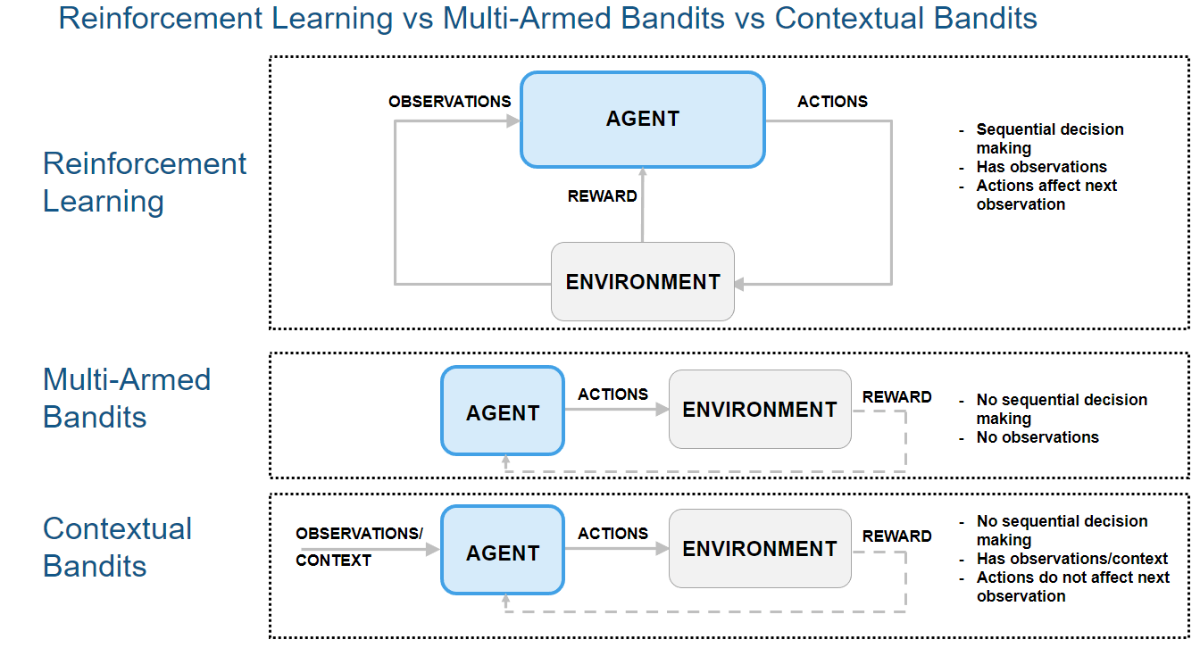
In bandit problems, the environment has no dynamics (that is, the state is constant and there are no state transitions), so the reward is only influenced by the current action and (for contextual bandits) the (constant) observation. In these problems the observation is also referred to as context. An alternative way to express the previous statements is that in contextual bandit problems an agent selects an action given the initial observation (context), it receives a reward, and the episode terminates.
Because neither rewards nor observations are influenced by previous actions or observations, the environment does not evolve along the time dimension, and there is no sequential decision making. The problem then becomes one of finding the action that maximizes the resulting immediate reward (given a context, if present). Single-armed bandit problems are just special cases of multi-armed bandit problems in which the action is a scalar instead of a vector.
The following figure shows how multi-armed bandits and contextual bandits are special cases of reinforcement learning problems.
Contextual bandits can be used for several applications such as hyperparameter tuning, recommender systems, medical treatment, and 5G communication.
Supervised learning problems can be also be recast as contextual bandit problems. For example, a classification problem can be recast as a contextual bandit problem in which the observation is an element that needs to be classified as belonging to a specific class, the action is the agent guess of the class to which belongs, and the corresponding reward indicates whether the agent's guess is correct or not.
Similarly, a regression problem in which a function needs to be approximated by a function of the parameter vector , can be recast as contextual bandit problem in which the observation is an element of the feasible domain of , is the action (the agent's guess of the value ), and the corresponding reward indicates how close is to , (for example, the reward could be ).
Since the reward (which can only be a scalar) intrinsically contains less information than the true class of (for the classification case) or than (for the regression case), you can generally expect training time to be considerably longer for the reinforcement learning case than for the corresponding supervised learning case. For examples discussing classification and regression as contextual bandit problems, see Why Solving Classification Using Reinforcement Learning Is Not Recommended and Why Solving Regression Using Reinforcement Learning is Not Recommended, respectively.
For more information on the relationship between reinforcement learning and supervised learning, see [2]. For a comprehensive introduction to bandit problems, see [3].
Fix Random Number Stream for Reproducibility
The example code might involve computation of random numbers at several stages. Fixing the random number stream at the beginning of some sections in the example code preserves the random number sequence in the section every time you run it, which increases the likelihood of reproducing the results. For more information, see Results Reproducibility. Fix the random number stream with seed 0 and random number algorithm Mersenne twister. For more information on controlling the seed used for random number generation, see rng.
previousRngState = rng(0,"twister");The output previousRngState is a structure that contains information about the previous state of the stream. You will restore the state at the end of the example.
Environment
The contextual bandit environment in this example is defined as follows:
Observation (discrete): {1, 2}
The context (initial observation) is sampled randomly.
Action (discrete): {1, 2, 3}
Reward:
Rewards in this environment are stochastic. The probability of each observation and action pair is defined as follows.
Note that the agent does not know these distributions.
Is-Done signal: Because this is a contextual bandit problem, each episode has only one step. Hence, the Is-Done signal is always 1.
Create Environment Object
The contextual bandit environment is implemented in the file ToyContextualBanditEnvironment, located in this example folder. For more information on how to implement a custom environment using the class template, see Create Custom Environment from Class Template.
Display the environment class. Note how the rewards are calculated in the environment step function, and how the observation (context) remains constant at its initial value.
type("ToyContextualBanditEnvironment.m")classdef ToyContextualBanditEnvironment < rl.env.MATLABEnvironment
%% Properties (set properties' attributes accordingly)
properties
% Initialize state
State = zeros(1,1)
end
properties(Access = protected)
% Initialize internal flag to indicate episode termination.
IsDone = false
end
%% Necessary Methods
methods
% Constructor method creates an instance of the environment.
% Change class name and constructor name accordingly.
function this = ToyContextualBanditEnvironment()
% Initialize Observation settings
% Observation = {s1, s2}, discrete
obsInfo = rlFiniteSetSpec([1 2]);
% Initialize Action settings
% Action = {a1, a2, a3}, discrete
actInfo = rlFiniteSetSpec([1 2 3]);
% Implement built-in functions of RL env
this = this@rl.env.MATLABEnvironment(obsInfo,actInfo);
end
% Apply system dynamics and simulate the environment
% with the given action for one step.
function [Observation,Reward,IsDone,aux] = step(this,Action)
aux = [];
% The action doesn't affect the next state
% in a contextual bandit problem.
Observation = this.State;
% Get reward
if this.State == 1
if Action == 1
% E(reward) = 2.9
if rand < 0.3
Reward = 5;
else
Reward = 2;
end
elseif Action == 2
% E(reward) = 1.9
if rand < 0.1
Reward = 10;
else
Reward = 1;
end
elseif Action == 3
% E(reward) = 3.5
Reward = 3.5;
end
elseif this.State == 2
if Action == 1
% E(reward) = 3.6
if rand < 0.2
Reward = 10;
else
Reward = 2;
end
elseif Action == 2
% E(reward) = 3.0
Reward = 3.0;
elseif Action == 3
% E(reward) = 3
if rand < 0.5
Reward = 5;
else
Reward = 0.5;
end
end
end
% Get IsDone.
IsDone = true;
this.IsDone = IsDone;
% (Optional) Use notifyEnvUpdated to signal
% that the environment has been updated
% (e.g. to update visualization).
notifyEnvUpdated(this);
end
% Reset environment to initial state
% and output initial observation.
function InitialObservation = reset(this)
% Pr(s1) = 0.5, Pr(s2) = 0.5
InitialObservation = randi(2);
this.State = InitialObservation;
% (Optional) Use notifyEnvUpdated to signal
% that the environment has been updated
% (e.g. to update visualization).
notifyEnvUpdated(this);
end
end
%% Optional Methods (set methods' attributes accordingly)
methods
% (Optional) Visualization method
function plot(this)
% Update the visualization
envUpdatedCallback(this)
end
% (Optional) Properties validation through set methods
function set.State(this,state)
mustBeMember(state,[1,2])
this.State = state;
notifyEnvUpdated(this);
end
end
end
Create the environment object.
env = ToyContextualBanditEnvironment;
Get observation and action specification objects.
obsInfo = getObservationInfo(env);
actInfo = getActionInfo(env);
Create a DQN Agent
Create a DQN agent option object. For more information, see rlDQNAgentOptions.
agentOpts = rlDQNAgentOptions( ...
    UseDoubleDQN = false, ...
    TargetSmoothFactor = 1, ...
    TargetUpdateFrequency = 4, ...
    MiniBatchSize = 64, ...
    MaxMiniBatchPerEpoch = 2);
agentOpts.EpsilonGreedyExploration.EpsilonDecay = 0.0005;
To create an agent with default network structure, in which each hidden layer has 16 neurons, use rlAgentInitializationOptions.
initOpts = rlAgentInitializationOptions(NumHiddenUnit = 16);
Create a DQN agent. For more information, see rlDQNAgent.
dqnAgent = rlDQNAgent(obsInfo, actInfo, initOpts, agentOpts);
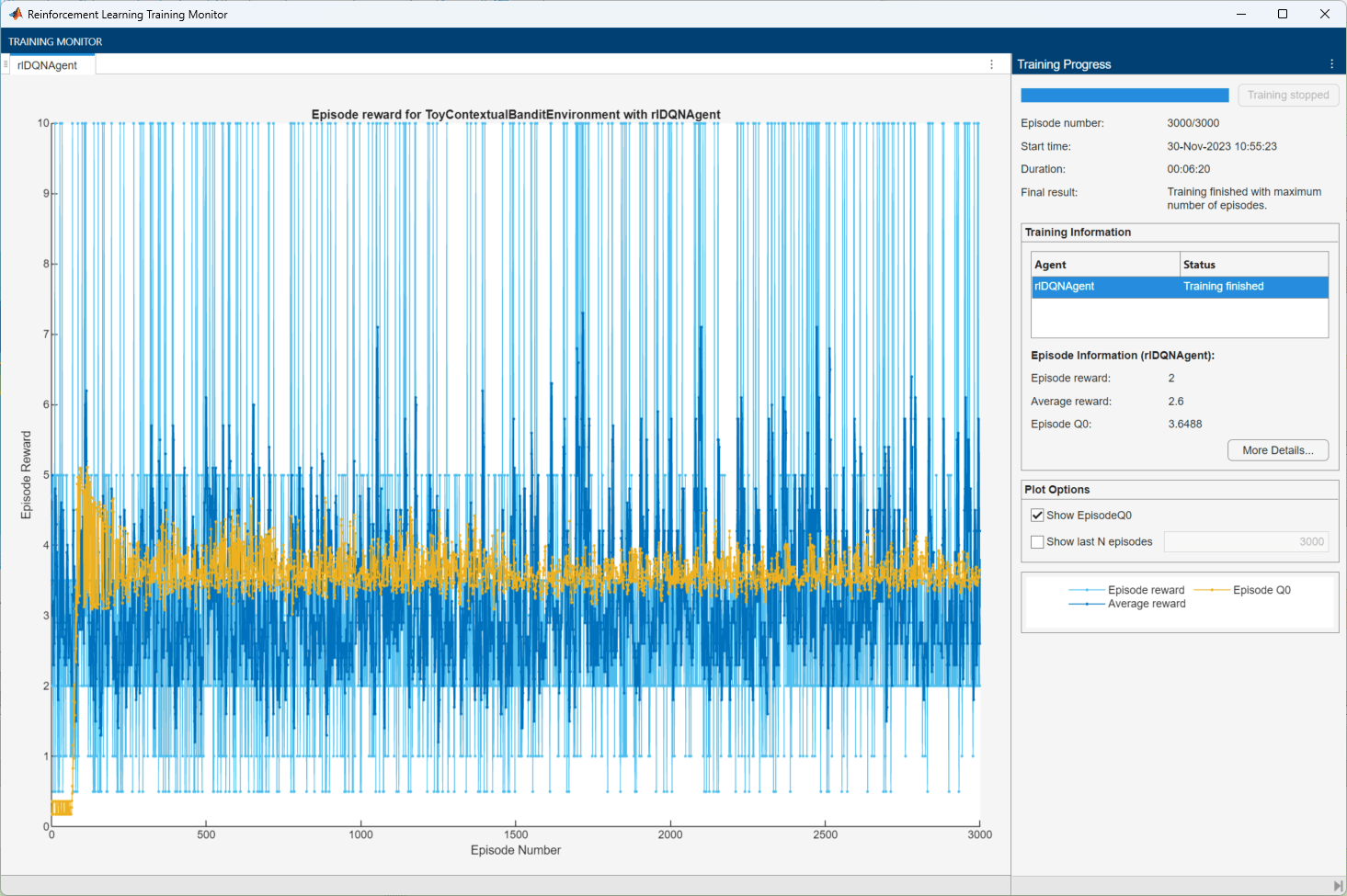
Train the DQN Agent
To train the agent, first specify the training options. For this example, use the following options:
Train for 3000 episodes.
Because this is a contextual bandit problem, and each episode has only one step, set
MaxStepsPerEpisodeto1.
For more information, see rlTrainingOptions.
trainOpts = rlTrainingOptions( ...
    MaxEpisodes=3000, ...
    MaxStepsPerEpisode=1, ...
    Verbose=false, ...
    Plots="training-progress", ...
    StopTrainingCriteria="None", ...
    StopTrainingValue="None");
Train the agent using the train function. Training is a computationally intensive process that takes several minutes to complete. To save time while running this example, load a pretrained agent by setting doTraining to false. To train the agent yourself, set doTraining to true.
doTraining =false; if doTraining % Train the agent trainingStats = train(dqnAgent,env,trainOpts); else % Load the pretrained agent for the example load("ToyContextualBanditDQNAgent.mat","dqnAgent") end
Validate the DQN Agent
For this example, you know the distribution of the rewards, and you can compute the optimal actions. Validate the agent's performance by comparing these optimal actions with the actions selected by the agent.
First, compute the true expected rewards using their true probability distribution.
1. The expected reward of each action at s=1 is as follows.
Hence, the optimal action is 3 when s=1.
2. The expected reward of each action at s=2 is as follows.
Hence, the optimal action is 1 when s=2.
With enough sampling, the Q-value estimates of the trained agent should be closer to the true expected reward.
Collect the true expected rewards in the ExpectedRewards variable.
ExpectedRewards = zeros(2,3);
ExpectedRewards(1,1) = 0.3*5 + 0.7*2;
ExpectedRewards(1,2) = 0.1*10 + 0.9*1;
ExpectedRewards(1,3) = 3.5;
ExpectedRewards(2,1) = 0.2*10 + 0.8*2;
ExpectedRewards(2,2) = 3.0;
ExpectedRewards(2,3) = 0.5*5 + 0.5*0.5;
Visualize the true expected rewards using the function localPlotQvalues defined at the end of the example.
localPlotQvalues(ExpectedRewards,"True Expected Rewards")
Now, validate whether the DQN agent learns the optimal behavior. Use getActionInfo to return the agent action given an input observation.
If the state is 1, the optimal action is 3.
observation = 1;
getAction(dqnAgent,observation)
ans = 1×1 cell array
    {[3]}
The agent selects the optimal action.
If the state is 2, the optimal action is 1.
observation = 2;
getAction(dqnAgent,observation)
ans = 1×1 cell array
    {[1]}
The agent selects the optimal action. Thus, the DQN agent has learned the optimal behavior.
Next, compare the Q-Value function to the true expected reward when selecting the optimal action.
Use getCritic to extract the critic from the trained agent, and getValue to return the value of an observation (using the learned value function).
dqnCritic = getCritic(dqnAgent);
qValues = zeros(2,3);
for s = 1:2
    qValues(s,:) = getValue(dqnCritic, {s});
end
Visualize the Q values for the DQN agent.
figure(1)
localPlotQvalues(qValues, "Q values of DQN agent")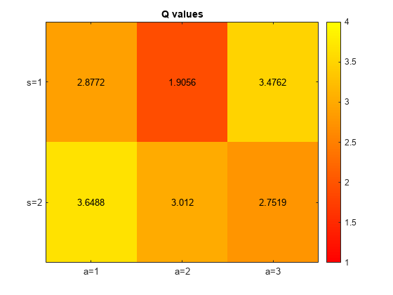
The learned Q-values are close to the true expected rewards computed above.
Create a Q-Learning Agent
Ensure reproducibility of the section by fixing the seed used for random number generation.
rng(0,"twister")For this example, use a table as approximation model for the critic.
Create a table using the observation and action specifications from the environment.
qTable = rlTable(obsInfo, actInfo);
Create an rlQValueFunction critic.
critic = rlQValueFunction(qTable, obsInfo, actInfo);
To set the agent exploration options, create an rlQAgentOptions object.
opt = rlQAgentOptions;
opt.EpsilonGreedyExploration.Epsilon = 1;
opt.EpsilonGreedyExploration.EpsilonDecay = 0.0005;
Create a Q agent. For more information, see rlQAgent.
qAgent = rlQAgent(critic,opt);
Train the Q-Learning Agent
To save time while running this example, load a pretrained agent by setting doTraining to false. To train the agent yourself, set doTraining to true.
doTraining =false; if doTraining % Train the agent. trainingStats = train(qAgent,env,trainOpts); else % Load the pretrained agent for the example. load("ToyContextualBanditQAgent.mat","qAgent") end

Validate the Q-Learning Agent
When the state is 1, the optimal action is 3.
observation = 1;
getAction(qAgent,observation)
ans = 1×1 cell array
    {[3]}
The agent selects the optimal action.
When the state is 2, the optimal action is 1.
observation = 2;
getAction(qAgent,observation)
ans = 1×1 cell array
    {[1]}
The agent selects the optimal action.
Next, compare the Q-Value function to the true expected reward when selecting the optimal action.
Use getCritic to extract the critic from the trained agent, and getValue to return the value of an observation (using the learned value function).
figure(2)
qCritic = getCritic(qAgent);
qValues = zeros(2,3);
for s = 1:2
    for a = 1:3
        qValues(s,a) = getValue(qCritic, {s}, {a});
    end
end
Visualize the Q values for the DQN agent.
localPlotQvalues(qValues, "Q values of Q agent")
The learned Q-values are close to the true expected rewards. The Q-values for deterministic rewards, Q(s=1, a=3) and Q(s=2, a=2), are the same as the true expected rewards.
Note that the corresponding Q-values learned by the DQN network, while close, are not identical to the true values. This happens because the DQN uses a neural network instead of a table as function approximation model.
Restore the random number stream using the information stored in previousRngState.
rng(previousRngState);
Local Function
function localPlotQvalues(QValues, titleText)
    % Visualize Q values
    figure;
    imagesc(QValues,[1,4])
    colormap("autumn")
    title(titleText)
    colorbar
    set(gca,"Xtick",1:3,"XTickLabel",{"a=1", "a=2", "a=3"})
    set(gca,"Ytick",1:2,"YTickLabel",{"s=1", "s=2"})

    % Plot values on the image
    x = repmat(1:size(QValues,2), size(QValues,1), 1);
    y = repmat(1:size(QValues,1), size(QValues,2), 1)';
    QValuesStr = num2cell(QValues);
    QValuesStr = cellfun(@num2str, QValuesStr, UniformOutput=false);
    text(x(:), y(:), QValuesStr, HorizontalAlignment = "Center")
end
Reference
[1] Sutton, Richard S., and Andrew G. Barto. Reinforcement Learning: An Introduction. Second edition. Adaptive Computation and Machine Learning Series. Cambridge, Massachusetts: The MIT Press, 2018.
[2] Barto, Andrew G., and Thomas G. Dietterich. Reinforcement Learning and its Relationship to Supervised Learning. https://all.cs.umass.edu/pubs/2004/barto_d_04.pdf.
[3] Slivkins, Aleksandrs. “Introduction to Multi-Armed Bandits.” arXiv, April 3, 2024. https://doi.org/10.48550/arXiv.1904.07272.
See Also
Apps
Functions
getActionInfo|train|sim
Objects
Topics
- Train Default DQN Agent to Balance Discrete Cart-Pole
- Why Solving Regression Using Reinforcement Learning is Not Recommended
- Why Solving Classification Using Reinforcement Learning Is Not Recommended
- Deep Q-Network (DQN) Agent
- Use Predefined Grid World Environments
- Train Reinforcement Learning Agents
- Create Actors, Critics, and Policy Objects