modelDiscrimination
Syntax
Description
DiscMeasure = modelDiscrimination(eadModel,data)modelDiscrimination supports segmentation and comparison
against a reference model and alternative methods to discretize the EAD response
into a binary variable.
[
specifies options using one or more name-value arguments in addition to the input
arguments in the previous syntax.DiscMeasure,DiscData] = modelDiscrimination(___,Name=Value)
Examples
This example shows how to use fitEADModel to create a Tobit model and then use modelDiscrimination to compute AUROC and ROC.
Load EAD Data
Load the EAD data.
load EADData.mat
head(EADData)
UtilizationRate Age Marriage Limit Drawn EAD
_______________ ___ ___________ __________ __________ __________
0.24359 25 not married 44776 10907 44740
0.96946 44 not married 2.1405e+05 2.0751e+05 40678
0 40 married 1.6581e+05 0 1.6567e+05
0.53242 38 not married 1.7375e+05 92506 1593.5
0.2583 30 not married 26258 6782.5 54.175
0.17039 54 married 1.7357e+05 29575 576.69
0.18586 27 not married 19590 3641 998.49
0.85372 42 not married 2.0712e+05 1.7682e+05 1.6454e+05
rng('default');
NumObs = height(EADData);
c = cvpartition(NumObs,'HoldOut',0.4);
TrainingInd = training(c);
TestInd = test(c);
Select Model Type
Select a model type for Tobit or Regression.
ModelType =  "Tobit";
Select Conversion Measure
Select a conversion measure for the EAD response values.
ConversionMeasure =  "LCF";
Create Tobit EAD Model
Use fitEADModel to create a Tobit model using the TrainingInd data.
eadModel = fitEADModel(EADData(TrainingInd,:),ModelType,PredictorVars={'UtilizationRate','Age','Marriage'}, ...
    ConversionMeasure=ConversionMeasure,DrawnVar="Drawn",LimitVar="Limit",ResponseVar="EAD");
disp(eadModel);
Tobit with properties:
CensoringSide: "both"
LeftLimit: 0
RightLimit: 1
ModelID: "Tobit"
Description: ""
UnderlyingModel: [1×1 risk.internal.credit.TobitModel]
PredictorVars: ["UtilizationRate" "Age" "Marriage"]
ResponseVar: "EAD"
LimitVar: "Limit"
DrawnVar: "Drawn"
ConversionMeasure: "lcf"
Display the underlying model. The underlying model's response variable is the transformation of the EAD response data. Use the 'LiimitVar' and 'DrwanVar' name-value arguments to modify the transformation.
disp(eadModel.UnderlyingModel);
Tobit regression model:
     EAD_lcf = max(0,min(Y*,1))
     Y* ~ 1 + UtilizationRate + Age + Marriage

Estimated coefficients:
                             Estimate         SE         tStat       pValue
                            __________    __________    _______    __________

    (Intercept)                0.22467      0.031504     7.1315    1.2783e-12
    UtilizationRate             0.4714       0.02066     22.817             0
    Age                     -0.0014209    0.00077019    -1.8449      0.065163
    Marriage_not married     -0.010543      0.015835    -0.6658        0.5056
    (Sigma)                     0.3618     0.0049955     72.426             0

Number of observations: 2627
Number of left-censored observations: 0
Number of uncensored observations: 2626
Number of right-censored observations: 1
Log-likelihood: -1057.9
Predict EAD
EAD prediction operates on the underlying compact statistical model and then transforms the predicted values back to the EAD scale. You can specify the predict function with different options for the 'ModelLevel' name-value argument.
predictedEAD = predict(eadModel,EADData(TestInd,:),ModelLevel="ead");
predictedConversion = predict(eadModel,EADData(TestInd,:),ModelLevel="ConversionMeasure");
Validate EAD Model
For model validation, use modelDiscrimination, modelDiscriminationPlot, modelCalibration, and modelCalibrationPlot.
Use modelDiscrimination and then modelDiscriminationPlot to plot the ROC curve.
ModelLevel = "ConversionMeasure";

[DiscMeasure1,DiscData1] = modelDiscrimination(eadModel,EADData(TestInd,:),ShowDetails=true,ModelLevel=ModelLevel)
"ConversionMeasure";
[DiscMeasure1,DiscData1] = modelDiscrimination(eadModel,EADData(TestInd,:),ShowDetails=true,ModelLevel=ModelLevel)DiscMeasure1=1×3 table
AUROC Segment SegmentCount
_______ __________ ____________
Tobit 0.70893 "all_data" 1751
DiscData1=1534×3 table
        X             Y           T
    __________    _________    _______

             0            0    0.63602
             0    0.0027778    0.63602
             0    0.0041667     0.6349
    0.00096993    0.0055556    0.63377
    0.00096993    0.0069444    0.63265
     0.0019399    0.0083333    0.63152
     0.0029098    0.0097222     0.6304
     0.0029098     0.015278    0.62927
     0.0029098     0.016667    0.62922
     0.0029098     0.018056     0.6288
     0.0029098     0.019444    0.62864
     0.0038797     0.022222    0.62814
     0.0038797        0.025    0.62767
     0.0048497     0.026389    0.62701
     0.0048497     0.033333    0.62654
     0.0058196     0.033333    0.62618
      ⋮
modelDiscriminationPlot(eadModel,EADData(TestInd,:),ModelLevel=ModelLevel,SegmentBy="Marriage");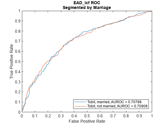
This example shows how to use fitEADModel to create a Beta model and then use modelDiscrimination to compute AUROC and ROC.
Load EAD Data
Load the EAD data.
load EADData.mat
head(EADData)
UtilizationRate Age Marriage Limit Drawn EAD
_______________ ___ ___________ __________ __________ __________
0.24359 25 not married 44776 10907 44740
0.96946 44 not married 2.1405e+05 2.0751e+05 40678
0 40 married 1.6581e+05 0 1.6567e+05
0.53242 38 not married 1.7375e+05 92506 1593.5
0.2583 30 not married 26258 6782.5 54.175
0.17039 54 married 1.7357e+05 29575 576.69
0.18586 27 not married 19590 3641 998.49
0.85372 42 not married 2.0712e+05 1.7682e+05 1.6454e+05
rng('default');
NumObs = height(EADData);
c = cvpartition(NumObs,'HoldOut',0.4);
TrainingInd = training(c);
TestInd = test(c);
Select Model Type
Select a model type for a Beta model.
ModelType =  "Beta";
Select Conversion Measure
Select a conversion measure for the EAD response values.
ConversionMeasure =  "LCF";
Create Beta EAD Model
Use fitEADModel to create a Beta model using the TrainingInd data.
eadModel = fitEADModel(EADData(TrainingInd,:),ModelType,PredictorVars={'UtilizationRate','Age','Marriage'}, ...
    ConversionMeasure=ConversionMeasure,DrawnVar="Drawn",LimitVar="Limit",ResponseVar="EAD");
disp(eadModel);
Beta with properties:
BoundaryTolerance: 1.0000e-07
ModelID: "Beta"
Description: ""
UnderlyingModel: [1×1 risk.internal.credit.BetaModel]
PredictorVars: ["UtilizationRate" "Age" "Marriage"]
ResponseVar: "EAD"
LimitVar: "Limit"
DrawnVar: "Drawn"
ConversionMeasure: "lcf"
Display the underlying model. The underlying model's response variable is the transformation of the EAD response data. Use the 'LiimitVar' and 'DrwanVar' name-value arguments to modify the transformation.
disp(eadModel.UnderlyingModel);
Beta regression model:
     logit(EAD_lcf) ~ 1_mu + UtilizationRate_mu + Age_mu + Marriage_mu
     log(EAD_lcf) ~ 1_phi + UtilizationRate_phi + Age_phi + Marriage_phi

Estimated coefficients:
                                Estimate        SE         tStat        pValue
                                _________    _________    ________    __________

    (Intercept)_mu               -0.65566      0.11484     -5.7093    1.2614e-08
    UtilizationRate_mu             1.7014     0.078094      21.787             0
    Age_mu                       -0.00559    0.0027603     -2.0252      0.042952
    Marriage_not married_mu     -0.012576     0.052098     -0.2414       0.80926
    (Intercept)_phi              -0.50132     0.094625     -5.2979    1.2685e-07
    UtilizationRate_phi           0.39731     0.066707       5.956    2.9304e-09
    Age_phi                     -0.001167    0.0023161    -0.50386       0.61441
    Marriage_not married_phi    -0.013275     0.042627    -0.31143        0.7555

Number of observations: 2627
Log-likelihood: -3140.21
Predict EAD
EAD prediction operates on the underlying compact statistical model and then transforms the predicted values back to the EAD scale. You can specify the predict function with different options for the 'ModelLevel' name-value argument.
predictedEAD = predict(eadModel,EADData(TestInd,:),ModelLevel="ead");
predictedConversion = predict(eadModel,EADData(TestInd,:),ModelLevel="ConversionMeasure");
Validate EAD Model
For model validation, use modelDiscrimination, modelDiscriminationPlot, modelCalibration, and modelCalibrationPlot.
Use modelDiscrimination and then modelDiscriminationPlot to plot the ROC curve.
ModelLevel = "ConversionMeasure";

[DiscMeasure1,DiscData1] = modelDiscrimination(eadModel,EADData(TestInd,:),ShowDetails=true,ModelLevel=ModelLevel)
"ConversionMeasure";
[DiscMeasure1,DiscData1] = modelDiscrimination(eadModel,EADData(TestInd,:),ShowDetails=true,ModelLevel=ModelLevel)DiscMeasure1=1×3 table
AUROC Segment SegmentCount
_______ __________ ____________
Beta 0.70895 "all_data" 1751
DiscData1=1534×3 table
        X             Y           T
    __________    _________    _______

             0            0    0.71675
             0    0.0027778    0.71675
             0    0.0041667    0.71561
             0    0.0055556    0.71533
    0.00096993    0.0069444    0.71447
    0.00096993    0.0097222    0.71419
    0.00096993     0.011111    0.71333
    0.00096993     0.018056    0.71304
     0.0019399     0.018056     0.7128
     0.0029098     0.019444    0.71218
     0.0048497     0.019444     0.7119
     0.0058196     0.020833    0.71104
     0.0067895     0.020833    0.71075
     0.0067895     0.022222    0.71022
     0.0067895     0.027778    0.70989
     0.0067895     0.029167    0.70968
      ⋮
modelDiscriminationPlot(eadModel,EADData(TestInd, :),ModelLevel=ModelLevel,SegmentBy="Marriage");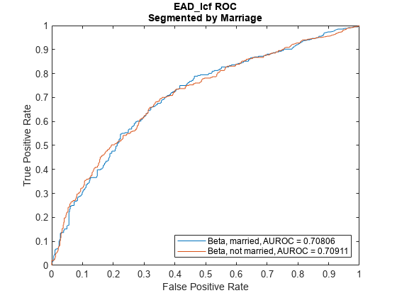
Input Arguments
Name-Value Arguments
Output Arguments
More About
References
[1] Baesens, Bart, Daniel Roesch, and Harald Scheule. Credit Risk Analytics: Measurement Techniques, Applications, and Examples in SAS. Wiley, 2016.
[2] Bellini, Tiziano. IFRS 9 and CECL Credit Risk Modelling and Validation: A Practical Guide with Examples Worked in R and SAS. San Diego, CA: Elsevier, 2019.
[3] Brown, Iain. Developing Credit Risk Models Using SAS Enterprise Miner and SAS/STAT: Theory and Applications. SAS Institute, 2014.
[4] Roesch, Daniel and Harald Scheule. Deep Credit Risk. Independently published, 2020.