interp1
Syntax
Description
vq = interp1(x,v,xq)x specifies the sample
points, and v specifies the quaternions that contains the
corresponding values v(x). xq specifies the query
points. By default, the function uses "slerp-short" interpolation
method.
vq = interp1(v,xq)v:
When
vis a vector of quaternions, the default points are1:length(v).When
vis an array of quaternions, the default points are1:size(v,1).
Use this syntax when you are not concerned about the absolute distances between sample points.
vq = interp1(v,xq,method,extrapolation)
Examples
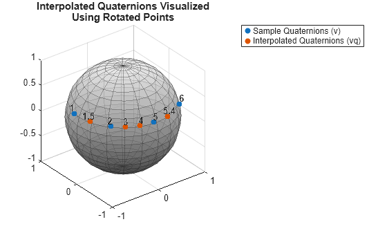
Define the sample points x and corresponding sample values v.
x = [1 2 5 6];
eul = [-185:45:-50; -20*ones(1,4); zeros(1,4)]';
v = quaternion(eul,"eulerd","ZYX","frame");
Define the query points over the range of x.
xq = [1.5 3 4 5.4];
Interpolate at the query points.
vq = interp1(x,v,xq);
To visualize the result, rotate the same point using the sample and interpolated quaternions.
pts_samples = rotatepoint(v,[1.05 0 0]);
pts_query = rotatepoint(vq,[1.05 0 0]);
Plot a unit sphere, and then plot the sample and interpolated quaternions on the sphere.
figure
[X,Y,Z] = sphere;
surf(X,Y,Z,FaceAlpha=0.5,EdgeAlpha=0.35)
colormap gray
hold on
scatter3(pts_samples(:,1),pts_samples(:,2),pts_samples(:,3),"filled")
scatter3(pts_query(:,1),pts_query(:,2),pts_query(:,3),"filled")
exampleHelperAnnotateQuats(pts_samples,pts_query,x,xq,10,1.05)
axis equal
title(["Interpolated Quaternions Visualized","Using Rotated Points"])
legend("","Sample Quaternions (v)","Interpolated Quaternions (vq)")
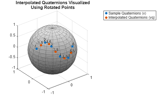
Define a set of function values.
eul = [-170:20:-70; -20*sind(0:72:360)-25; zeros(1,6)]';
v = quaternion(eul,"eulerd","ZYX","frame");
Define a set of query points that fall between the default points, 1:6. In this case, the default points are 1:6 because v is a six-element quaternion array.
xq = [1.5 2.6 3.5 4.5 5.5];
Evaluate v at xq using the SQUAD natural interpolation method. Note that you could use the default "slerp-short" interpolation method here, but for the sine-wave rotation that this quaternion function describes, SQUAD produces a smoother interpolated path.
vq = interp1(v,xq,"squad-natural");To visualize the result, rotate a point on the x-axis using the sample and interpolated quaternions.
pts_samples = rotatepoint(v,[1.05 0 0]);
pts_query = rotatepoint(vq,[1.05 0 0]);
Plot a unit sphere, and then plot the sample and interpolated quaternions on the sphere.
figure
[X,Y,Z] = sphere;
surf(X,Y,Z,FaceAlpha=0.5,EdgeAlpha=0.35)
colormap gray
hold on
scatter3(pts_samples(:,1),pts_samples(:,2),pts_samples(:,3),"filled")
scatter3(pts_query(:,1),pts_query(:,2),pts_query(:,3),"filled")
exampleHelperAnnotateQuats(pts_samples,pts_query,1:6,xq,9,1.05)
axis equal
title(["Interpolated Quaternions Visualized","Using Rotated Points"])
legend("","Sample Quaternions (v)","Interpolated Quaternions (vq)")
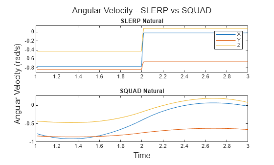
Define three quaternions representing different orientations.
q0 = quaternion([0 0 0],"euler","ZYX","frame");
q1 = quaternion([pi/4 pi/6 pi/3],"euler","ZYX","frame");
q2 = quaternion([pi/2 pi/4 pi/2],"euler","ZYX","frame");
Create a time vector for the original keyframes
x = [1 2 3];
Create a time vector for interpolation
T = linspace(0,3,300);
Interpolate using interp1 with the "slerp-natural" and "squad-natural" methods.
quats_slerp = interp1(x,[q0 q1 q2],T,"slerp-natural")';
quats_squad = interp1(x,[q0 q1 q2],T,"squad-natural")';
Calculate the angular velocities for both interpolations methods.
ang_vel_slerp = angvel(quats_slerp,T(2)-T(1),"frame");
ang_vel_squad = angvel(quats_squad,T(2)-T(1),"frame");
Plot the angular velocities.
tl = tiledlayout(2,1);
title(tl,"Angular Velocity - SLERP vs SQUAD")
Plot the angular velocities for the SLERP and SQUAD interpolations. Note that the angular velocity from the SQUAD interpolation is smoother than the interpolation using SLERP.
nexttile
plot(T,ang_vel_slerp)
ylim padded
title("SLERP Natural")
legend("X","Y","Z")
nexttile
plot(T,ang_vel_squad)
ylim padded
title("SQUAD Natural")
xlabel(tl,"Time")
ylabel(tl,"Angular Velocity (rad/s)")
Define the sample points x and corresponding sample values v.
x = [0 1 2];
eul = [0 30 60; 0 20 60; zeros(1,3)]';
v = quaternion(eul,"eulerd","ZYX","frame");
Specify the query points xq so that they extend beyond the domain of x.
xq = [-0.5 0.5 1.5 2.5];
Now evaluate v at xq using the "slerp-short" interpolation method, and assign any values outside the domain of x to a quaternion with all parts set to 0.
vq = interp1(x,v,xq,"slerp-short",ones("quaternion"))'
vq = 4×1 quaternion array
            1 +        0i +        0j +        0k
      0.98774 + 0.022751i - 0.084907j -  0.12903k
      0.87097 +    0.151i -  0.30755j -  0.35217k
            1 +        0i +        0j +        0k
Input Arguments
Output Arguments
Algorithms
References
[1] Shoemake, Ken. "Animating Rotation with Quaternion Curves." ACM SIGGRAPH Computer Graphics 19, no. 3 (July 1985): 245–54. https://doi.org/10.1145/325165.325242.
[2] Dam, Erik B., Martin Koch, and Martin Lillholm. Quaternions, Interpolation and Animation. Technical Report DIKU-TR-98/5. Department of Computer Science, University of Copenhagen, July 17, 1998. https://web.mit.edu/2.998/www/QuaternionReport1.pdf.
Extended Capabilities
Version History
Introduced in R2025a