Create Models of Uncertain Systems

Forms of model uncertainty include:

• Uncertainty in parameters of the underlying differential equation models

• Frequency-domain uncertainty, which often quantifies model uncertainty by describing absolute or relative uncertainty in the process's frequency response

Using these two basic building blocks, along with conventional system creation commands (such as ss and tf), you can easily create uncertain system models.

Creating Uncertain Parameters

An uncertain parameter has a name (used to identify it within an uncertain system with many uncertain parameters) and a nominal value. Being uncertain, it also has variability, described in one of the following ways:

• An additive deviation from the nominal

• A range about the nominal

• A percentage deviation from the nominal

Create a real parameter, with name '|bw|', nominal value 5, and a percentage uncertainty of 10%.

bw = ureal('bw',5,'Percentage',10)

Uncertain real parameter "bw" with nominal value 5 and variability [-10,10]%.

This command creates a ureal object that stores a number of parameters in its properties. View the properties of bw.

get(bw)

    NominalValue: 5
            Mode: 'Percentage'
           Range: [4.5000 5.5000]
       PlusMinus: [-0.5000 0.5000]
      Percentage: [-10 10]
    AutoSimplify: 'basic'
            Name: 'bw'

Note that the range of variation (Range property) and the additive deviation from nominal (the PlusMinus property) are consistent with the Percentage property value.

You can create state-space and transfer function models with uncertain real coefficients using ureal objects. The result is an uncertain state-space (uss) object. As an example, use the uncertain real parameter bw to model a first-order system whose bandwidth is between 4.5 and 5.5 rad/s.

H = tf(1,[1/bw 1])

Uncertain continuous-time state-space model with 1 outputs, 1 inputs, 1 states.
The model uncertainty consists of the following blocks:
  bw: Uncertain real, nominal = 5, variability = [-10,10]%, 1 occurrences

Type "H.NominalValue" to see the nominal value and "H.Uncertainty" to interact with the uncertain elements.

Note that the result H is an uncertain system, called a uss model. The nominal value of H is a state-space (ss) model. Verify that the pole is at -5, as expected from the uncertain parameter's nominal value of 5.

pole(H.NominalValue)

ans = -5

Next, use bodeplot and stepplot to examine the behavior of H. These commands plot the responses of the nominal system and a number of random samples of the uncertain system.

bodeplot(H,{1e-1 1e2});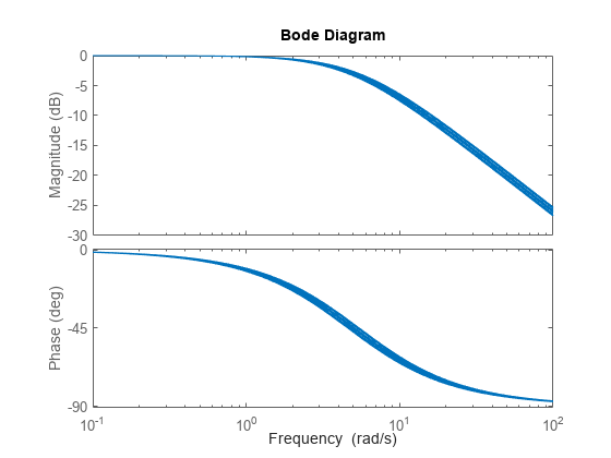

stepplot(H)

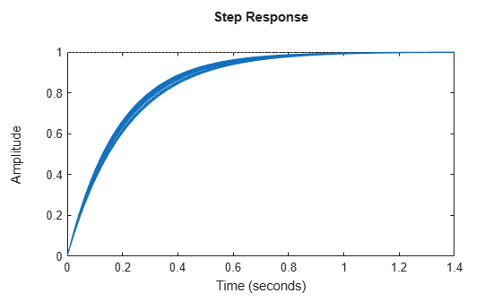
While there are variations in the bandwidth and time constant of H, the high-frequency rolls off at 20 dB/decade regardless of the value of bw. You can capture the more complicated uncertain behavior that typically occurs at high frequencies using the ultidyn uncertain element.

Quantifying Unmodeled Dynamics

An informal way to describe the difference between the model of a process and the actual process behavior is in terms of bandwidth. It is common to hear “The model is good out to 8 radians/second.” The precise meaning is not clear, but it is reasonable to believe that for frequencies lower than, say, 5 rad/s, the model is accurate, and for frequencies beyond, say, 30 rad/s, the model is not necessarily representative of the process behavior. In the frequency range between 5 and 30, the guaranteed accuracy of the model degrades.

The uncertain linear, time-invariant dynamics object ultidyn can be used to model this type of knowledge. An ultidyn object represents an unknown linear system whose only known attribute is a uniform magnitude bound on its frequency response. When coupled with a nominal model and a frequency-shaping filter, ultidyn objects can be used to capture uncertainty associated with the model dynamics.

Suppose that the behavior of the system modeled by H significantly deviates from its first-order behavior beyond 9 rad/s, for example, about 5% potential relative error at low frequency, increasing to 1000% at high frequency where H rolls off. In order to model frequency domain uncertainty as described above using ultidyn objects, follow these steps:

1. Create the nominal system Gnom, using tf, ss, or zpk. Gnom itself might already have parameter uncertainty. In this case Gnom is H, the first-order system with an uncertain time constant.

2. Create a filter W, called the “weight,” whose magnitude represents the relative uncertainty at each frequency. The utility makeweight is useful for creating first-order weights with specific low- and high-frequency gains, and specified gain crossover frequency.

3. Create an ultidyn object Delta with magnitude bound equal to 1.

The uncertain model G is formed by G = Gnom*(1+W*Delta).

If the magnitude of W represents an absolute (rather than relative) uncertainty, use the formula G = Gnom + W*Delta instead.

The following commands carry out these steps:

bw = ureal('bw',5,'Percentage',10);
H = tf(1,[1/bw 1]);

Gnom = H;
W = makeweight(.05,9,10);
Delta = ultidyn('Delta',[1 1]);
G = Gnom*(1+W*Delta)

Uncertain continuous-time state-space model with 1 outputs, 1 inputs, 2 states.
The model uncertainty consists of the following blocks:
  Delta: Uncertain 1x1 LTI, peak gain = 1, 1 occurrences
  bw: Uncertain real, nominal = 5, variability = [-10,10]%, 1 occurrences

Type "G.NominalValue" to see the nominal value and "G.Uncertainty" to interact with the uncertain elements.

Note that the result G is also an uncertain system, with dependence on both Delta and bw. You can use bode to make a Bode plot of 20 random samples of G's behavior over the frequency range [0.1 100] rad/s.

bode(G,{1e-1 1e2})

Gain and Phase Uncertainty

A special case of dynamic uncertainty is uncertainty in the gain and phase in a feedback loop. Modeling gain and phase variations in your uncertain system model lets you verify stability margins during robustness analysis or enforce them during robust controller design. Use the umargin control design block to represent gain and phase variations in feedback loops. For more information, see Uncertain Gain and Phase.

Related Topics

• System with Uncertain Parameters
• Systems with Unmodeled Dynamics
• Model Gain and Phase Uncertainty in Feedback Loops

×

Apri esempio

Si dispone di una versione modificata di questo esempio. Desideri aprire questo esempio con le tue modifiche?

No, sovrascrivi la versione modificata Sì