Generate a Presentation From the Results of a MATLAB Application

Open Live Script

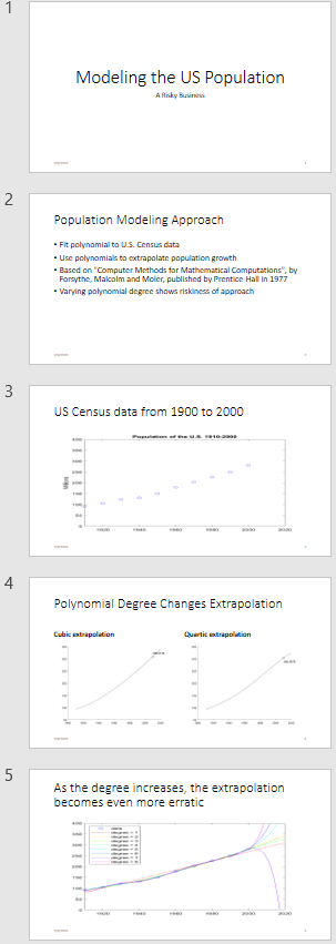
This example shows how to use the MATLAB® API for PowerPoint® (PPT API) to generate a Microsoft® PowerPoint® presentation from the results of a MATLAB application. The example generates a presentation from the results of an application that predicts the United States population. Here are the slides that the example generates:

Create the Presentation

Import the PPT namespace so that you do not have to use long, fully qualified names.

import mlreportgen.ppt.*;

To facilitate deleting the images that the example generates, create a cell array to hold the images.

images = {};

Create a presentation, using the default template.

ppt = Presentation('population.pptx');
open(ppt);

Add Slides to the Presentation

PowerPoint presentations consist of slides that are created from predefined layouts. The layouts contain placeholders that you fill with generated content. The predefined layouts belong to a template slide master that defines the styles.

Add the first slide to the presentation, using the Title Slide layout.

slide1 = add(ppt,'Title Slide');

Replace the title and subtitle in the slide by using the replace method.

replace(slide1,'Title','Modeling the US Population');
replace(slide1,'Subtitle','A Risky Business');

Add the second slide to the presentation using the Title and Content layout. Replace the title.

slide2 = add(ppt,'Title and Content');
replace(slide2,'Title','Population Modeling Approach');

Add text to the Content placeholder using a cell array.

replace(slide2,'Content',{ ...
    'Fit polynomial to U.S. Census data' ...
    'Use polynomials to extrapolate population growth' ...
    ['Based on "Computer Methods for Mathematical Computations",'...
   ' by Forsythe, Malcolm and Moler, published by Prentice-Hall in 1977'] ...
    'Varying polynomial degree shows riskiness of approach'});

Add the third slide to the presentation using the Title and Content layout. Replace the title.

slide3 = add(ppt,'Title and Content');
replace(slide3,'Title','US Census data from 1900 to 2000');

Create a plot of US census data from 1910 to 2000.

% Time interval
t = (1910:10:2000)';

% Population
p = [91.972 105.711 123.203 131.669 150.697...
    179.323 203.212 226.505 249.633 281.422]';

% Plot
fig1 = figure;
plot(t,p,'bo');
axis([1910 2020 0 400]);
title('Population of the U.S. 1910-2000');
ylabel('Millions');

Convert the plot to an image. Add the image to the list of images to be deleted at the end of presentation generation. You must not delete the images until after you close the presentation.

img1 = 'plot1.png';
saveas(fig1,img1);

Figure contains an axes object. The axes object with title Population of the U.S. 1910-2000, ylabel Millions contains a line object which displays its values using only markers.

images = [images {img1}];

Replace the Content placeholder with the image.

replace(slide3,'Content',Picture(img1));

Add the fourth slide to the presentation using the Comparison layout. Use this slide to show a comparison of the cubic and quartic extrapolations of the population data.

slide4 = add(ppt,'Comparison');
replace(slide4,'Title','Polynomial Degree Changes Extrapolation');

Compute the coefficients for a polynomial approximation of the population data.

n = length(t);
s = (t-1950)/50;
A = zeros(n);
A(:,end) = 1;
for j = n-1:-1:1
    A(:,j) = s .* A(:,j+1);
end
c = A(:,n-3:n)\p;

Replace the Left Text placeholder with text.

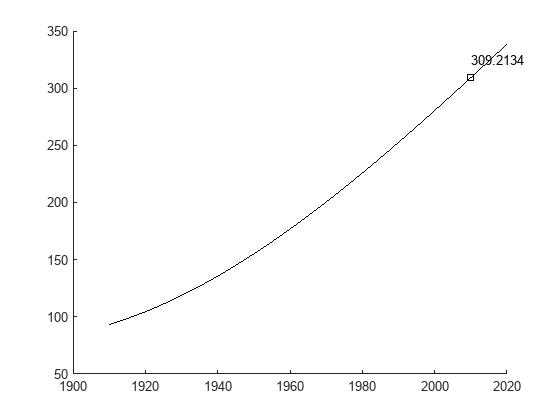
replace(slide4,'Left Text','Cubic extrapolation');

Compute the cubic extrapolation.

v = (1910:2020)';
x = (v-1950)/50;
w = (2010-1950)/50;
y = polyval(c,x);
z = polyval(c,w);

fig2 = figure;
hold on
plot(v,y,'k-');
plot(2010,z,'ks');
text(2010,z+15,num2str(z));
hold off

Create an image from the plot and add the image to the list of images to be deleted.

img2 = 'plot2.png';
saveas(fig2,img2);

Figure contains an axes object. The axes object contains 3 objects of type line, text. One or more of the lines displays its values using only markers

images = [images {img2}];

Replace the Left Content placeholder with the image.

replace(slide4,'Left Content',Picture(img2));

Replace the Right Text placeholder with text.

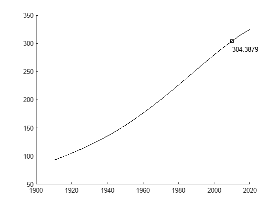
replace(slide4,'Right Text','Quartic extrapolation');

Compute the quartic extrapolation.

c = A(:,n-4:n)\p;
y = polyval(c,x);
z = polyval(c,w);
fig3 = figure;
hold on
plot(v,y,'k-');
plot(2010,z,'ks');
text(2010,z-15,num2str(z));
hold off

Create an image from the plot, add the image to the list of images to be deleted, and replace the Right Content placeholder with the image.

img3 = 'plot3.png';
saveas(fig3,img3);

Figure contains an axes object. The axes object contains 3 objects of type line, text. One or more of the lines displays its values using only markers

images = [images {img3}];
replace(slide4,'Right Content',Picture(img3));

Add the last slide to the presentation using the Title and Content layout.

slide5 = add(ppt,'Title and Content');
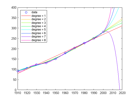
replace(slide5,'Title','As the degree increases, the extrapolation becomes even more erratic');

Create a plot to demonstrate that as the degree increases, the extrapolation becomes even more erratic.

fig4 = figure;
cla
plot(t,p,'bo')
hold on
axis([1910 2020 0 400])
colors = hsv(8);
labels = {'data'};
for d = 1:8
   [Q,R] = qr(A(:,n-d:n));
   R = R(1:d+1,:);
   Q = Q(:,1:d+1);
   c = R\(Q'*p);   
   y = polyval(c,x);
   z = polyval(c,11);
   plot(v,y,'color',colors(d,:));
   labels{end+1} = ['degree = ' int2str(d)];
end
legend(labels, 'Location', 'NorthWest')
hold off

Create an image from the plot and replace the Content placeholder with the image.

img4 = 'plot4.png';
saveas(fig4,img4);

Figure contains an axes object. The axes object contains 9 objects of type line. One or more of the lines displays its values using only markers These objects represent data, degree = 1, degree = 2, degree = 3, degree = 4, degree = 5, degree = 6, degree = 7, degree = 8.

images = [images {img4}];
replace(slide5,'Content',Picture(img4));

Close and View the Presentation

close(ppt);
rptview(ppt);

Delete the Images

When the presentation closes, the images are copied into the presentation. Now, you can delete the images.

len = length(images);
for i = 1:len
    delete(images{i});
end

Generate a Presentation From the Results of a MATLAB Application

Create the Presentation

Add Slides to the Presentation

Close and View the Presentation

Delete the Images

See Also

Related Topics