findsignal
Find signal location using similarity search
Syntax
Description
[
returns the start and stop indices of a segment of the data array,
istart,istop
,dist
]
= findsignal(data
,signal
)data
, that best matches the search array,
signal
. The best-matching segment is such that
dist
, the squared Euclidean distance between the
segment and the search array, is smallest. If data
and
signal
are matrices, then findsignal
finds the start and end columns of the region of data
that
best matches signal
. In that case,
data
and signal
must have the same
number of rows.
[
specifies
additional options using name-value pair arguments. Options include
the normalization to apply, the number of segments to report, and
the distance metric to use.istart,istop
,dist
]
= findsignal(data
,signal
,Name,Value
)
findsignal(___)
without output
arguments plots data
and highlights any identified
instances of signal
.
If the arrays are real vectors, the function displays
data
as a function of sample number.If the arrays are complex vectors, the function displays
data
on an Argand diagram.If the arrays are real matrices, the function uses
imagesc
to displaysignal
on a subplot anddata
with the highlighted regions on another subplot.If the arrays are complex matrices, the function plots their real and imaginary parts in the top and bottom half of each image.
Examples
Locate Signal in Data
Generate a data set consisting of a 5 Hz Gaussian pulse with 50% bandwidth, sampled for half a second at a rate of 1 kHz.
fs = 1e3; t = 0:1/fs:0.5; data = gauspuls(t,5,0.5);
Create a signal consisting of one-and-a-half cycles of a 10 Hz sinusoid. Plot the data set and the signal.
ts = 0:1/fs:0.15; signal = cos(2*pi*10*ts); subplot(2,1,1) plot(t,data) title('Data') subplot(2,1,2) plot(ts,signal) title('Signal')
Find the segment of the data that has the smallest squared Euclidean distance to the signal. Plot the data and highlight the segment.
figure findsignal(data,signal)
Add two clearly outlying sections to the data set. Find the segment that is closest to the signal in the sense of having the smallest absolute distance.
dt = data; dt(t>0.31&t<0.32) = 2.1; dt(t>0.32&t<0.33) = -2.1; findsignal(dt,signal,'Metric','absolute')
Let the x-axes stretch if the stretching results in a smaller absolute distance between the closest data segment and the signal.
findsignal(dt,signal,'TimeAlignment','dtw','Metric','absolute')
Add two more outlying sections to the data set.
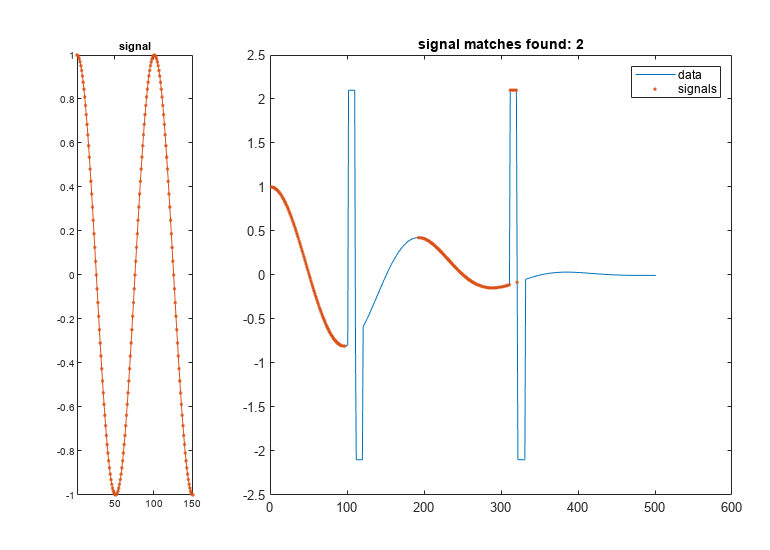
dt(t>0.1&t<0.11) = 2.1; dt(t>0.11&t<0.12) = -2.1; findsignal(dt,signal,'TimeAlignment','dtw','Metric','absolute')
Find the two data segments closest to the signal.
findsignal(dt,signal,'TimeAlignment','dtw','Metric','absolute', ... 'MaxNumSegments',2)
Go back to finding one segment. Choose 'edr'
as the x-axis stretching criterion. Select an edit distance tolerance of 3. The edit distance between nonmatching samples is independent of the actual separation, making 'edr'
robust to outliers.
findsignal(dt,signal,'TimeAlignment','edr','EDRTolerance',3, ... 'Metric','absolute')
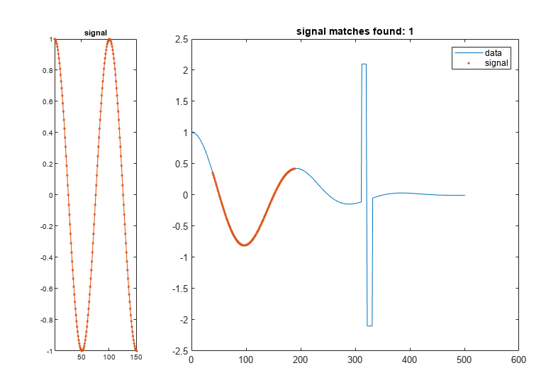
Repeat the calculation, but now normalize the data and the signal.
Define a moving window with 10 samples to either side of each data and signal point.
Subtract the mean of the data in the window and divide by the local standard deviation.
Find the normalized data segment that has the smallest absolute distance to the normalized signal. Display the unnormalized and normalized versions of the data and the signal.
findsignal(dt,signal,'TimeAlignment','edr','EDRTolerance',3, ... 'Normalization','zscore','NormalizationLength',21, ... 'Metric','absolute','Annotate','all')
Find Signal in Data with Abrupt Changes
Generate a random data array where:
The mean is constant in each of seven regions and changes abruptly from region to region.
The standard deviation is constant in each of five regions and changes abruptly from region to region.
lr = 20; mns = [0 1 4 -5 2 0 1]; nm = length(mns); vrs = [1 4 6 1 3]/2; nv = length(vrs); v = randn(1,lr*nm*nv); f = reshape(repmat(mns,lr*nv,1),1,lr*nm*nv); y = reshape(repmat(vrs,lr*nm,1),1,lr*nm*nv); t = v.*y+f;
Plot the data, highlighting the steps of its construction. Display the mean and standard deviation of each region.
subplot(2,2,1) plot(v) title('Original') xlim([0 700]) subplot(2,2,2) plot([f;v+f]') title('Means') xlim([0 700]) text(lr*nv*nm*((0:1/nm:1-1/nm)+1/(2*nm)), ... -7*ones(1,nm),num2str(mns'), ... 'HorizontalAlignment',"center") subplot(2,2,3) plot([y;v.*y]') title('STD') xlim([0 700]) text(lr*nv*nm*((0:1/nv:1-1/nv)+1/(2*nv)), ... -7*ones(1,nv),num2str(vrs'), ... 'HorizontalAlignment',"center") subplot(2,2,4) plot(t) title('Final') xlim([0 700])
Create a random signal with a mean of zero and a standard deviation of 1/2. Find and display the segment of the data array that best matches the signal.
sg = randn(1,2*lr)/2; findsignal(t,sg)
Create a random signal with a mean of zero and a standard deviation of 2. Find and display the segment of the data array that best matches the signal.
sg = randn(1,2*lr)*2; findsignal(t,sg)
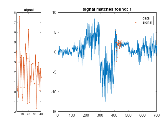
Create a random signal with a mean of 2 and a standard deviation of 2. Find and display the segment of the data array that best matches the signal.
sg = randn(1,2*lr)*2+2; findsignal(t,sg)
Create a random signal with a mean of -4 and a standard deviation of 3. Find and display the segment of the data array that best matches the signal.
sg = randn(1,2*lr)*3-4; findsignal(t,sg)
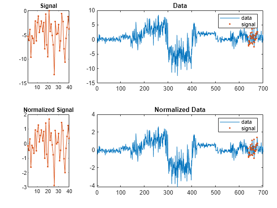
Repeat the calculation, but this time subtract the mean from both the signal and the data.
findsignal(t,sg,Normalization="zscore",Annotate="all")
Find Letter in Writing Sample
Devise a typeface that resembles the output of early computers. Use it to write the word MATLAB®.
rng default
chr = @(x)dec2bin(x')-48;
M = chr([34 34 54 42 34 34 34]);
A = chr([08 20 34 34 62 34 34]);
T = chr([62 08 08 08 08 08 08]);
L = chr([32 32 32 32 32 32 62]);
B = chr([60 34 34 60 34 34 60]);
MATLAB = [M A T L A B];
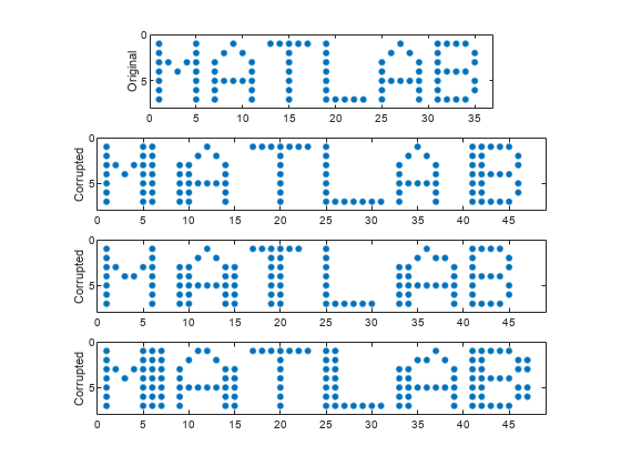
Corrupt the word by repeating random columns of the letters and varying the spacing. Show the original word and three corrupted versions.
c = @(x)x(:,sort([1:6 randi(6,1,2)])); subplot(4,1,1,'XLim',[0 60]) spy(MATLAB) xlabel('') ylabel('Original') for kj = 2:4 subplot(4,1,kj,'XLim',[0 60]) spy([c(M) c(A) c(T) c(L) c(A) c(B)]) xlabel('') ylabel('Corrupted') end
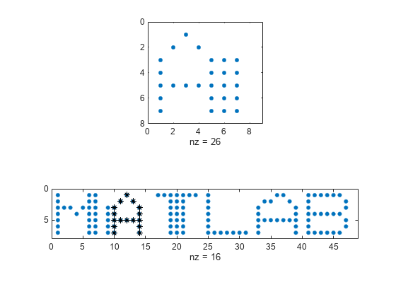
Generate one more corrupted version of the word. Search for a noisy version of the letter "A." Display the distance between the search array and the data segment closest to it. The segment spills into the "T" because the horizontal axes are rigid.
corr = [c(M) c(A) c(T) c(L) c(A) c(B)]; sgn = c(A); [ist,ind,dst] = findsignal(corr,sgn); clf subplot(2,1,1) spy(sgn) subplot(2,1,2) spy(corr) chk = zeros(size(corr)); chk(:,ist:ind) = corr(:,ist:ind); hold on spy(chk,'*k') hold off
dst
dst = 11
Allow the horizontal axes to stretch. The closest segment is the intersection of the search array and the first instance of "A." The distance between the segment and the array is zero.
[ist,ind,dst] = findsignal(corr,sgn,'TimeAlignment','dtw'); subplot(2,1,1) spy(sgn) subplot(2,1,2) spy(corr) chk = zeros(size(corr)); chk(:,ist:ind) = corr(:,ist:ind); hold on spy(chk,'*k') hold off
dst
dst = 0
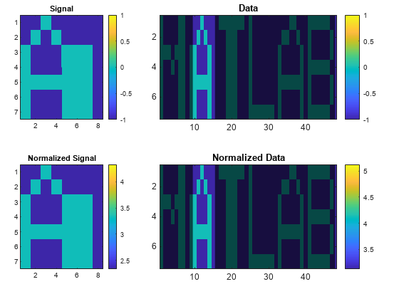
Repeat the computation using the built-in functionality of findsignal
. Divide by the local mean to normalize the data and the signal. Use the symmetric Kullback-Leibler metric.
findsignal(corr,sgn,'TimeAlignment','dtw', ... 'Normalization','power','Metric','symmkl','Annotate','all')
Input Arguments
data
— Data array
vector | matrix
Data array, specified as a vector or matrix.
Data Types: single
| double
Complex Number Support: Yes
signal
— Search array
vector | matrix
Search array, specified as a vector or matrix.
Data Types: single
| double
Complex Number Support: Yes
Name-Value Arguments
Specify optional pairs of arguments as
Name1=Value1,...,NameN=ValueN
, where Name
is
the argument name and Value
is the corresponding value.
Name-value arguments must appear after other arguments, but the order of the
pairs does not matter.
Before R2021a, use commas to separate each name and value, and enclose
Name
in quotes.
Example: 'MaxNumSegments',2,'Metric','squared','Normalization','center','NormalizationLength',11
finds
the two segments of the data array that have the smallest squared
Euclidean distances to the search signal. Both the data and the signal
are normalized by subtracting the mean of a sliding window. The window
has five samples to either side of each point, for a total length
of 5 + 5 + 1 = 11 samples.
Normalization
— Normalization statistic
'none'
(default) | 'center'
| 'power'
| 'zscore'
Normalization statistic, specified as the comma-separated pair
consisting of 'Normalization'
and one of these
values:
'none'
— Do not normalize.'center'
— Subtract local mean.'power'
— Divide by local mean.'zscore'
— Subtract local mean and divide by local standard deviation.
NormalizationLength
— Normalization length
length(data)
(default) | integer scalar
Normalization length, specified as the comma-separated pair
consisting of 'NormalizationLength'
and an integer
scalar. This value represents the minimum number of samples over which
to normalize each sample in both the data and the signal. If the signal
is a matrix, then 'NormalizationLength'
represents a
number of columns.
Data Types: single
| double
MaxDistance
— Maximum segment distance
Inf
(default) | positive real scalar
Maximum segment distance, specified as the comma-separated pair consisting
of 'MaxDistance'
and a positive real scalar. If
you specify 'MaxDistance'
, then findsignal
returns
the start and stop indices of all segments of data
whose
distances from signal
are both local minima and
smaller than 'MaxDistance'
.
Data Types: single
| double
MaxNumSegments
— Maximum number of segments to return
1
(default) | positive integer scalar
Maximum number of segments to return, specified as the comma-separated
pair consisting of 'MaxNumSegments'
and a positive
integer scalar. If you specify 'MaxNumSegments'
,
then findsignal
locates all segments of data
whose
distances from the signal are local minima and returns up to 'MaxNumSegments'
segments
with smallest distances.
Data Types: single
| double
TimeAlignment
— Time alignment technique
'fixed'
(default) | 'dtw'
| 'edr'
Time alignment technique, specified as the comma-separated pair
consisting of 'TimeAlignment'
and one of these
values:
'fixed'
— Do not stretch or repeat samples to minimize the distance.'dtw'
— Attempt to reduce the distance by stretching the time axis and repeating samples in either the data or the signal. Seedtw
for more information.'edr'
— Minimize the number of edits so that the distance between each remaining sample of the data segment and its signal counterpart lies within a given tolerance. An edit consists of removing a sample from the data, the signal, or both. Specify the tolerance using the'EDRTolerance'
argument. Use this option when any of the input arrays has outliers. Seeedr
for more information.
EDRTolerance
— Edit distance tolerance
real scalar
Edit distance tolerance, specified as the comma-separated pair
consisting of 'EDRTolerance'
and a real scalar.
Use this argument to find the signal when the 'TimeAlignment'
name-value
pair argument is set to 'edr'
.
Data Types: single
| double
Metric
— Distance metric
'squared'
(default) | 'absolute'
| 'euclidean'
| 'symmkl'
Distance metric, specified as the comma-separated pair consisting of
'Metric'
and one of 'squared'
,
'absolute'
, 'euclidean'
, or
'symmkl'
. If X
and Y are both
K-dimensional signals, then
Metric
prescribes
dmn(X,Y), the
distance between the mth sample of X and the nth sample of
Y. See Dynamic Time Warping for more
information about
dmn(X,Y).
'squared'
— Square of the Euclidean metric, consisting of the sum of squared differences:'euclidean'
— Root sum of squared differences, also known as the Euclidean or ℓ2 metric:'absolute'
— Sum of absolute differences, also known as the Manhattan, city block, taxicab, or ℓ1 metric:'symmkl'
— Symmetric Kullback-Leibler metric. This metric is valid only for real and positive X and Y:
Annotate
— Plot style
'signal'
(default) | 'data'
| 'all'
Plot style, specified as the comma-separated pair consisting
of 'Annotate'
and one of these values:
'data'
plots the data and highlights the regions that best match the signal.'signal'
plots the signal in a separate subplot.'all'
plots the signal, the data, the normalized signal, and the normalized data in separate subplots.
This argument is ignored if you call findsignal
with
output arguments.
Output Arguments
istart,istop
— Segment start and end indices
integer scalars | vectors
Segment start and end indices, returned as integer scalars or vectors.
dist
— Minimum data-signal distance
scalar | vector
Minimum data-signal distance, returned as a scalar or a vector.
Extended Capabilities
C/C++ Code Generation
Generate C and C++ code using MATLAB® Coder™.
Version History
Introduced in R2016b
MATLAB Command
You clicked a link that corresponds to this MATLAB command:
Run the command by entering it in the MATLAB Command Window. Web browsers do not support MATLAB commands.
Select a Web Site
Choose a web site to get translated content where available and see local events and offers. Based on your location, we recommend that you select: .
You can also select a web site from the following list
How to Get Best Site Performance
Select the China site (in Chinese or English) for best site performance. Other MathWorks country sites are not optimized for visits from your location.
Americas
- América Latina (Español)
- Canada (English)
- United States (English)
Europe
- Belgium (English)
- Denmark (English)
- Deutschland (Deutsch)
- España (Español)
- Finland (English)
- France (Français)
- Ireland (English)
- Italia (Italiano)
- Luxembourg (English)
- Netherlands (English)
- Norway (English)
- Österreich (Deutsch)
- Portugal (English)
- Sweden (English)
- Switzerland
- United Kingdom (English)
Asia Pacific
- Australia (English)
- India (English)
- New Zealand (English)
- 中国
- 日本Japanese (日本語)
- 한국Korean (한국어)