sbioensembleplot
Show results of ensemble run using 2-D or 3-D plots
Syntax
sbioensembleplot(simdataObj)

sbioensembleplot(simdataObj, Names)

sbioensembleplot(simdataObj, Names, Time)


FH = sbioensembleplot(simdataObj, Names)

FH = sbioensembleplot(simdataObj, Names, Time)
Arguments
| An object that contains simulation data. You can generate a sbioensemblerun. All elements
of |
| Character vector, string, string vector, string array, or cell array of character vectors.
'
or
'
to resolve ambiguities. Specifying {} or
empty string array (string.empty) for
|
| A numeric scalar value. If the specified |
| Array of handles to figure windows. |
Description
sbioensembleplot( shows
a 3-D shaded plot of time-varying distribution of all logged states
in the SimData array simdataObj)simdataObjsbioensemblerun function plots an approximate
distribution created by fitting a normal distribution to the data
at every time step.
sbioensembleplot( plots
the distribution for the data specified by simdataObj, Names)Names
sbioensembleplot( plots
a 2-D histogram of the actual data of the ensemble distribution of
the states specified by simdataObj, Names, Time)NamesTime
returns
an array of handles FH = sbioensembleplot(simdataObj, Names)FH
FH = sbioensembleplot(simdataObj, Names, Time)FH
Examples
This example shows how to plot data from an ensemble run without interpolation.
Get Statistics from Ensemble Run of SimBiology Model
Load the radiodecay model.
sbioloadproject("radiodecay.sbproj");Change the solver of the active configuration set to be ssa. Also, adjust the LogDecimation property on the SolverOptions property of the configuration set.
cs = getconfigset(m1,"active");
cs.SolverType = "ssa";
so = cs.SolverOptions;
so.LogDecimation = 10;
Perform an ensemble of 20 runs with no interpolation.
ensembleData = sbioensemblerun(m1,20);
sbioensembleplot(ensembleData, 'z', 1.0);
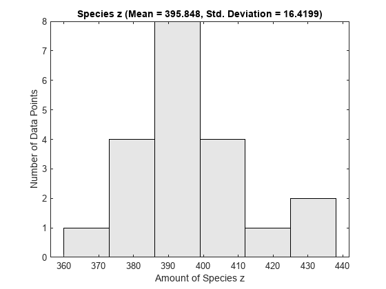
Create a 2-D distribution plot of the species z at time = 1.0.
sbioensembleplot(ensembleData,"z",1.0); 
Get ensemble statistics for all species using the default interpolation method.
[T,M,V] = sbioensemblestats(ensembleData);
Get ensemble statistics for a specific species using the default interpolation scheme.
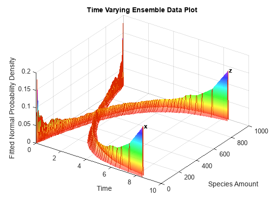
[T2,M2,V2] = sbioensemblestats(ensembleData,"z");Create a 3-D shaded plot of the species x and z.
sbioensembleplot(ensembleData,["x","z"]);

Version History
Introduced in R2006a