Estimate Frequency Response Models with Noise Using Signal Processing Toolbox
Open the Simulink® model, and specify which portion of the model to linearize:
load_system('magball')
io(1) = linio('magball/Desired Height',1);
io(2) = linio('magball/Magnetic Ball Plant',1,'output');
Create a random input signal for simulation:
in = frest.Random('Ts',0.001,'NumSamples',1e4);
Linearize the model at a steady-state operating point:
op = findop('magball',operspec('magball'),...
            findopOptions('DisplayReport','off'));
sys = linearize('magball',io,op);
Simulate the model to obtain the output at the linearization output point:
[sysest,simout] = frestimate('magball',io,in,op);Estimate a frequency response model using Signal Processing Toolbox™ software, which includes windowing and averaging:
input = generateTimeseries(in);
output = detrend(simout{1}.Data,'constant');
[Txy,F] = tfestimate(input.Data(:),...
          output,hanning(4000),[],4000,1/in.Ts);
systfest = frd(Txy,2*pi*F);
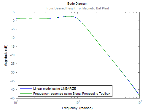
Compare the results of analytical linearization and tfestimate (Signal Processing Toolbox):
ax = axes;
h = bodeplot(ax,sys,'b',systfest,'g',systfest.Frequency);
setoptions(h,'Xlim',[10,1000],'PhaseVisible','off')
legend(ax,'Linear model using LINEARIZE','Frequency response using Signal Processing Toolbox',...
			'Location','SouthWest')

In this case, the Signal Processing Toolbox command tfestimate (Signal Processing Toolbox) gives a more accurate estimation
than frestimate due to windowing
and averaging.