Frequency-Dependent Transmission Line
This example shows a custom frequency-dependent transmission line model. The characteristic admittance and propagation function are first derived from the frequency-dependent resistance, reactance, and susceptance. The derived values are fitted using RF Toolbox. The Universal Line Model (ULM) [1] is then implemented in Simscape based on the fitted parameters. The results from the frequency-dependent transmission line model and the classic pi-section transmission line model are compared.
Model

Specification of Parameters
Import the frequency-dependent parameters of the transmission line. These parameters are computed for an overhead line that is 20 m above the ground [2]. The ground resistivity and the skin effect of the conductor are considered negligible. The following parameters are pre-computed for the simulation:
Frequency-dependent series resistance per unit length,

Frequency-dependent series reactance per unit length,

Frequency-dependent shunt susceptance per unit length,

Corresponding frequency,

Length of the transmission line,

  Name         Size            Bytes  Class     Attributes

  B         1000x1              8000  double
  R         1000x1              8000  double
  X         1000x1              8000  double
  freq      1000x1              8000  double
  len          1x1                 8  double
The frequency-dependent R, L and C are shown in these figures:

Characteristic Admittance and Propagation Function
The characteristic admittance is expressed as  , where
  and
and  are the frequency-dependent series impedance and shunt admittance per unit length.
The propagation velocity is expressed as:  , where
  is the propagation constant, and
  is the corresponding angular velocity.
The propagation function,  , is then expressed as
  .
.
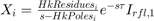
Rational Fitting for Characteristic Admittance
To convert the characteristic admittance to the rational form, use the rational fit function rationalfit (RF Toolbox) from RF Toolbox.
where:
 is the number of poles (order of the fit).
 is the
  pole of
  .
. is the residue of .
In this case, an eighth order fit is performed.
These figures show the comparison between the characteristic admittance before and after rational fitting.

Rational Fitting for Propagation Function
The time delay of the propagation function is first removed to help reduce the order of rational fitting, where  is the propagation time delay and
  is the propagation function without time delay. The time delay is represented by a delay unit in the model.

To convert the propagation function without time delay to the rational form, use the rationalfit (RF Toolbox) function from RF Toolbox.
where:
- is the number of poles (order of the fit).
 is the pole of .
 is the residue of .
In this case, an eighth order fit is performed.
These figures show that the propagation function H (with time delay) before and after rational fitting agree.

Universal Line Model Implemented in Simscape
In this example, only a single conductor and the ground return is considered. The equivalent circuit of the line in Laplace domain can be deduced from the Universal Line Model (ULM) [1]. Key variables are:
 is the voltage at terminal
  .
. is the current at terminal .
 is the shunt current at terminal .
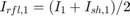
 is the reflected current from terminal .
 is the auxiliary current from terminal .
- is the propagation function.

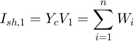
From this equivalent circuit, the system of equations can be written as:
where:


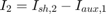
Considering the rational form of the characteristic admittance, the shunt current on terminal one is:
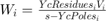
To transform these equations from Laplace domain to time domain, an inverse Laplace transform is performed. This transformation leads to:
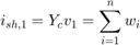

where  ,
,  and
and  are the time domain representation of
  ,
,  and
and  .
.
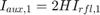
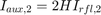
Similarly, considering the rational form of the propagation function, the auxiliary current on terminal one is:

To transform these equations from Laplace domain to time domain, an inverse Laplace transform is performed. This transformation leads to:


Currents on terminal two can be deduced using the same procedure. Time domain equations are then implemented in Simscape using Simscape™ language.
Simulation Results from Simscape Logging
For the first simulation case, the voltage source is generating a 60 Hz sine wave. The Pi-Section Transmission Line uses an RLC parameterized assuming a 60 Hz input, which matches the frequency of the voltage source. The plot shows the input and output terminal voltages of the transmission line. The two models show good agreement at steady state.

For the second simulation case, the voltage source is generating a 60 Hz sine wave with a 10 kHz modulation. The Pi-Section Transmission Line still uses an RLC parameterized assuming a 60 Hz input. It is clear that the custom frequency-dependent transmission line model is suitable for broader band signals whereas the pi-section model is only applicable for extremely narrow band signals.

References
[1] Morched, Atef, Bjorn Gustavsen, and Manoocher Tartibi. "A universal model for accurate calculation of electromagnetic transients on overhead lines and underground cables." IEEE Transactions on Power Delivery 14.3 (1999): 1032-1038.
[2] Dommel, Herman W. "Overhead line parameters from handbook formulas and computer programs." IEEE Transactions on Power Apparatus and Systems 2 (1985): 366-372.
See Also
Simscape Component | Transmission Line | Circuit Breaker | SFFM Voltage Source | rationalfit (RF Toolbox)