Block Coordinate Descent Approximation for GPR Models
For a large number of observations, using the exact method for parameter estimation
and making predictions on new data can be expensive (see Exact GPR Method). One of the approximation methods that help deal with
this issue for prediction is the Block Coordinate Descent (BCD) method. You can make
predictions using the BCD method by first specifying the predict method using the
PredictMethod="bcd" name-value argument in the call to
fitrgp, and then using the predict function.
The idea of the BCD method is to compute
in a different way than the exact method. BCD estimates by solving the following optimization problem:
where
fitrgp uses block coordinate descent (BCD) to solve the above
optimization problem. For users familiar with support vector machines (SVMs), sequential
minimal optimization (SMO) and ISDA (iterative single data algorithm) used to fit SVMs
are special cases of BCD. fitrgp performs two steps for each BCD
update - block selection and block update. In the block selection phase,
fitrgp uses a combination of random and greedy strategies for
selecting the set of coefficients to optimize next. In the block update phase, the selected coefficients are optimized while keeping the other coefficients fixed to their previous values. These two steps are
repeated until convergence. BCD does not store the matrix in memory but it just computes chunks of the matrix as needed. As a result BCD is more memory efficient compared to
PredictMethod="exact".
Practical experience indicates that it is not necessary to solve the optimization
problem for computing to very high precision. For example, it is reasonable to stop the
iterations when drops below , where is the initial value of and is a small constant (say ). The results from PredictMethod="exact" and
PredictMethod="bcd" are equivalent except BCD computes in a different way. Hence, PredictMethod="bcd" can
be thought of as a memory efficient way of doing
PredictMethod="exact". BCD is often faster than
PredictMethod="exact" for large n. However,
you cannot compute the prediction intervals using the
PredictMethod="bcd" option. This is because computing prediction
intervals requires solving a problem like the one solved for computing for every test point, which again is expensive.
Fit GPR Models Using BCD Approximation
This example shows fitting a Gaussian Process Regression (GPR) model to data with a large number of observations, using the Block Coordinate Descent (BCD) Approximation.
Small n - PredictMethod "exact" and "bcd" Produce the Same Results
Generate a small sample data set.
rng(0,"twister")
n = 1000;
X = linspace(0,1,n)';
X = [X,X.^2];
y = 1 + X*[1;2] + sin(20*X*[1;-2])./(X(:,1)+1) + 0.2*randn(n,1);
Create a GPR model using FitMethod="exact" and PredictMethod="exact".
gpr = fitrgp(X,y,KernelFunction="squaredexponential", ...
    FitMethod="exact",PredictMethod="exact");
Create another GPR model using FitMethod="exact" and PredictMethod="bcd".
gprbcd = fitrgp(X,y,KernelFunction="squaredexponential", ...
    FitMethod="exact",PredictMethod="bcd",BlockSize=200);
PredictMethod="exact" and PredictMethod="bcd" should be equivalent. They compute the same but just in different ways. You can also see the iterations by using the Verbose=1 name-value argument in the call to fitrgp.
Compute the fitted values using the two methods and compare them.
ypred = resubPredict(gpr);
ypredbcd = resubPredict(gprbcd);
max(abs(ypred-ypredbcd))
ans = 5.8853e-04
The fitted values are close to each other.
Now, plot the data along with fitted values for PredictMethod="exact" and PredictMethod="bcd".
figure
plot(y,".")
hold on
plot(ypred,"-",LineWidth=2)
plot(ypredbcd,"--",LineWidth=2)
hold off
legend("Data","PredictMethod Exact","PredictMethod BCD", ...
    Location="best")
xlabel("Observation index")
ylabel("Response value")
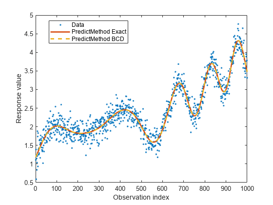
It can be seen that PredictMethod="exact" and PredictMethod="bcd" produce nearly identical fits.
Large n - Use FitMethod="sd" and PredictMethod="bcd"
Generate a bigger data set similar to the previous one.
rng(0,"twister")
n = 50000;
X = linspace(0,1,n)';
X = [X,X.^2];
y = 1 + X*[1;2] + sin(20*X*[1;-2])./(X(:,1)+1) + 0.2*randn(n,1);
For n = 50000, the matrix K(X, X) would be 50000-by-50000. Storing K(X, X) in memory would require around 20 GB of RAM. To fit a GPR model to this data set, use FitMethod="sd" with a random subset of m = 2000 points. The ActiveSetSize name-value argument in the call to fitrgp specifies the active set size m. For computing , use PredictMethod="bcd" with a BlockSize of 5000. The BlockSize name-value argument in fitrgp specifies the number of elements of the vector that the software optimizes at each iteration. A BlockSize of 5000 assumes that the computer you use can store a 5000-by-5000 matrix in memory.
gprbcd = fitrgp(X,y,KernelFunction="squaredexponential", ...
    FitMethod="sd",ActiveSetSize=2000,PredictMethod="bcd",BlockSize=5000);
Plot the data and the fitted values.
figure
plot(y,".")
hold on
plot(resubPredict(gprbcd),"-",LineWidth=2)
hold off
legend("Data","PredictMethod BCD",Location="best")
xlabel("Observation index")
ylabel("Response value")
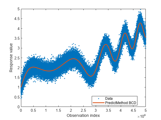
The plot is similar to the one for smaller n.
References
[1] Grippo, L. and M. Sciandrone. "On the convergence of the block nonlinear Gauss-Seidel method under convex constraints." Operations Research Letters. Vol. 26, pp. 127–136, 2000.
[2] Bo, L. and C. Sminchisescu. "Greed block coordinate descent for large scale Gaussian process regression." In Proceedings of the Twenty Fourth Conference on Uncertainty in Artificial Intelligence (UAI2008): http://arxiv.org/abs/1206.3238, 2012.