Exploratory Analysis of Data

Explore the distribution of data using visualizations and descriptive statistics. Compare the results to a normal distribution.

Generate Data

Generate a vector containing randomly generated sample data. Combine 100 random numbers, generated from the normal distribution with mean 4 and standard deviation 1, with 200 random numbers, generated from the normal distribution with mean 6 and standard deviation 0.5.

rng(0,"twister") % For reproducibility
x = [normrnd(4,1,1,100),normrnd(6,0.5,1,200)];

Visualize Data

Plot a histogram of the sample data with a normal density fit. The plot provides a visual comparison of the sample data and a normal distribution fitted to the data.

histfit(x)

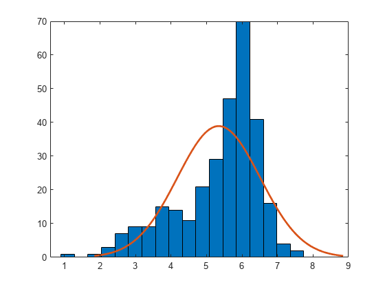
The distribution of the data appears to be left-skewed. A normal distribution does not look like a good fit for this sample data.

Create a normal probability plot. The plot provides another way to visually compare the sample data to a normal distribution fitted to the data.

probplot("normal",x)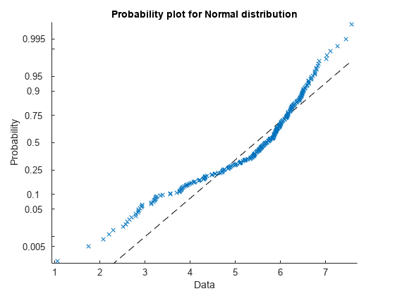

Because the plotted points do not appear along the reference line, the probability plot also shows the deviation of data from normality.

Create a box plot to visualize the statistics.

boxchart(x)

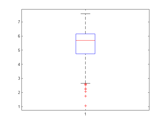
The box plot shows the 0.25, 0.5, and 0.75 quantiles. The line inside the box corresponds to the 0.5 quantile (median), while the top and bottom edges of the box correspond to the 0.25 and 0.75 quantiles, respectively. The long lower tail and circled points (outliers) show the lack of symmetry in the sample data values.

Compute Descriptive Statistics

Compute the mean and median of the data.

y1 = [mean(x),median(x)]

y1 = 1×2

    5.3438    5.6872

The mean and median values seem close to each other, but a mean smaller than the median usually indicates that the data is left-skewed.

Compute the skewness and kurtosis of the data.

y2 = [skewness(x),kurtosis(x)]

y2 = 1×2

   -1.0417    3.5895

A negative skewness value means the data is left-skewed. The data has a larger peakedness than a normal distribution because the kurtosis value is greater than 3.

Identify possible outliers by computing the z-scores and finding the values that are greater than 3 or less than -3.

z = zscore(x);
find(abs(z)>3)

ans = 1×2

     3    35

Based on the z-scores, the 3rd and 35th observations are potential outliers.