plotProfileLikelihood

Plot profile loglikelihood for nonlinear regression model

Since R2025a

collapse all in page

Syntax

plotProfileLikelihood(mdl,coef)

plotProfileLikelihood(mdl,coef,Name=Value)

plotProfileLikelihood(ax,___)

H = plotProfileLikelihood(___)

Description

plotProfileLikelihood(mdl,coef) plots the profile loglikelihood, Wald approximation, coefficient estimate, and likelihood-ratio and Wald confidence intervals for the model mdl and coefficient of interest coef.

example

plotProfileLikelihood(mdl,coef,Name=Value) specifies additional options using one or more name-value arguments. For example, you can specify the significance level for the confidence interval and the values for the coefficient of interest.

example

plotProfileLikelihood(ax,___) plots into the axes specified by ax instead of the current axes (gca), using any of the input argument combinations in the previous syntaxes.

H = plotProfileLikelihood(___) returns an array of Line objects for the lines in the plot.

example

Examples

collapse all

Plot Profile Loglikelihood

Open Live Script

Load a table of standardized variables generated from the carbig data set.

load standardizedcar.mat

The table tbl contains the variables Horsepower, Weight, and MPG, which represent car horsepower, weight, and miles per gallon, respectively.

Fit a nonlinear model to the data using Horsepower and Weight as predictors, and MPG as the response.

modelfun = @(b,x) exp(b(1)*x(:,1))+b(2)*x(:,2)+b(3);
beta0 = [0.01 2 -1];
mdl = fitnlm(tbl,modelfun,beta0)

mdl = 
Nonlinear regression model:
    MPG ~ exp(b1*Horsepower) + b2*Weight + b3

Estimated Coefficients:
          Estimate       SE        tStat       pValue   
          ________    ________    _______    ___________

    b1    -0.57016    0.045819    -12.444     3.7322e-30
    b2    -0.39274    0.043737    -8.9797     1.1804e-17
    b3     -1.1417    0.034105    -33.476    1.3291e-116


Number of observations: 392, Error degrees of freedom: 389
Root Mean Squared Error: 0.516
R-Squared: 0.735,  Adjusted R-Squared 0.733
F-statistic vs. constant model: 539, p-value = 8.27e-113

mdl contains a fitted nonlinear regression model. The coefficient b1 is a nonlinear coefficient because it is inside the exponential term in the model function.

Plot the profile loglikelihood, coefficient estimate, Wald approximation, and Wald and likelihood-ratio confidence intervals for b1.

plotProfileLikelihood(mdl,"b1")

Figure contains an axes object. The axes object with xlabel b1, ylabel log likelihood contains 5 objects of type line. One or more of the lines displays its values using only markers These objects represent Estimate, Exact log likelihood, Wald approximation, Wald interval, LR interval.

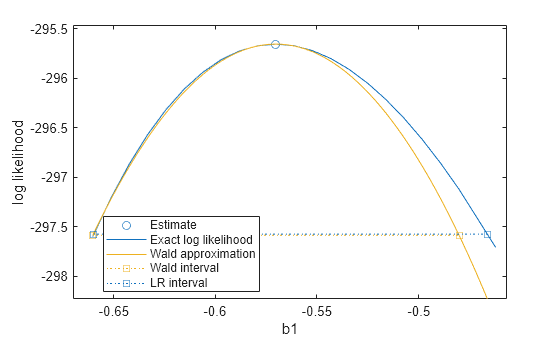
The plot shows that the maximum likelihood estimate for b1 appears at the peak of the profile loglikelihood, confirming it is the maximum likelihood estimate. The likelihood-ratio confidence interval is slightly wider than the Wald interval, and is also asymmetric. However, the closeness of the two intervals suggests that the assumptions of the Wald approximation hold true for this model.

Compare Profile Loglikelihoods

Open Live Script

Load a table of standardized variables generated from the carbig data set.

load standardizedcar.mat

The table tbl contains the variables Horsepower, Weight, and MPG, which represent car horsepower, weight, and miles per gallon, respectively.

Fit a nonlinear model to the data using car Horsepower and Weight as predictors, and MPG as the response.

modelfun = @(b,x) exp(b(1)*x(:,1))+b(2)*x(:,2)+b(3);
beta0 = [0.01 2 -1];
mdl = fitnlm(tbl,modelfun,beta0)

mdl = 
Nonlinear regression model:
    MPG ~ exp(b1*Horsepower) + b2*Weight + b3

Estimated Coefficients:
          Estimate       SE        tStat       pValue   
          ________    ________    _______    ___________

    b1    -0.57016    0.045819    -12.444     3.7322e-30
    b2    -0.39274    0.043737    -8.9797     1.1804e-17
    b3     -1.1417    0.034105    -33.476    1.3291e-116


Number of observations: 392, Error degrees of freedom: 389
Root Mean Squared Error: 0.516
R-Squared: 0.735,  Adjusted R-Squared 0.733
F-statistic vs. constant model: 539, p-value = 8.27e-113

mdl contains a fitted nonlinear regression model.

Plot the profile loglikelihoods for the coefficients without plotting the likelihood-ratio confidence intervals.

tiledlayout(3,1)
nexttile
plotProfileLikelihood(mdl,"b1",ShowInterval=0)
nexttile
plotProfileLikelihood(mdl,"b2",ShowInterval=0)
nexttile
plotProfileLikelihood(mdl,"b3",ShowInterval=0)

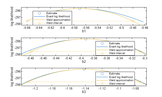
The plots show that the profile loglikelihoods are smooth and appear quadratic in nature. Near the coefficient estimates, the Wald intervals are quadratic estimations of the loglikelihood function, so they follow the profile loglikelihood closely.

Modify Line Properties

Open Live Script

Load a table of standardized variables generated from the carbig data set.

load standardizedcar.mat

The table tbl contains the variables Horsepower, Weight, and MPG, which represent car horsepower, weight, and miles per gallon, respectively.

Fit a nonlinear model to the data using Horsepower and Weight as predictors, and MPG as the response.

modelfun = @(b,x) exp(b(1)*x(:,1))+b(2)*x(:,2)+b(3);
beta0 = [0.01 2 -1];
mdl = fitnlm(tbl,modelfun,beta0)

mdl = 
Nonlinear regression model:
    MPG ~ exp(b1*Horsepower) + b2*Weight + b3

Estimated Coefficients:
          Estimate       SE        tStat       pValue   
          ________    ________    _______    ___________

    b1    -0.57016    0.045819    -12.444     3.7322e-30
    b2    -0.39274    0.043737    -8.9797     1.1804e-17
    b3     -1.1417    0.034105    -33.476    1.3291e-116


Number of observations: 392, Error degrees of freedom: 389
Root Mean Squared Error: 0.516
R-Squared: 0.735,  Adjusted R-Squared 0.733
F-statistic vs. constant model: 539, p-value = 8.27e-113

mdl contains a fitted nonlinear regression model.

Generate an array of Line objects representing the coefficient estimate, profile loglikelihood, Wald approximation, and 99% Wald and likelihood-ratio confidence intervals for the coefficient b2.

H = plotProfileLikelihood(mdl,"b2",Alpha=0.01)

H = 
  1×5 Line array:

    Line    Line    Line    Line    Line

H contains five Line objects.

Plot the coefficient estimate in green, the profile loglikelihood and likelihood-ratio interval in black, and the Wald approximation and confidence interval in magenta.

H(1).MarkerFaceColor="g"; % Confidence estimate
H(1).MarkerEdgeColor="g";
H(2).Color = "k"; % Profile loglikelihood
H(3).Color = "k"; % Likelihood-ratio confidence interval
H(4).Color = "m"; % Wald approximation
H(5).Color = "m"; % Wald confidence interval

Figure contains an axes object. The axes object with xlabel b2, ylabel log likelihood contains 5 objects of type line. One or more of the lines displays its values using only markers These objects represent Estimate, Exact log likelihood, Wald approximation, Wald interval, LR interval.

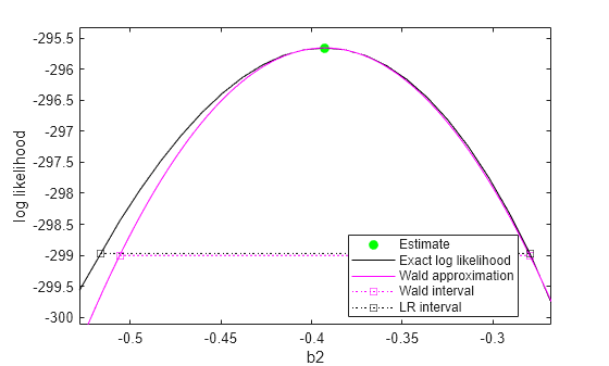
The plot shows that the maximum likelihood estimate for b2 appears at the peak of the profile loglikelihood, confirming it is the maximum likelihood estimate. The likelihood-ratio confidence interval is slightly wider than the Wald interval, and is also asymmetric. However, the closeness of the two intervals suggests that the assumptions of the Wald approximation hold true for this model.

Input Arguments

collapse all

`mdl` — Nonlinear regression model
`NonLinearModel` object

Nonlinear regression model, specified as a NonLinearModel object created using fitnlm.

`coef` — Coefficient of interest
string | character array | index

Coefficient of interest, specified as a string, character array, or index. Coefficients not specified in coef are called nuisance coefficients. For each value of the coefficient of interest, plotProfileLikelihood calculates values for the nuisance coefficients. For more information, see Profile Loglikelihood.

Example: "b1"

Example: 3

Data Types: single | double | char | string

`ax` — Target axes
`Axes` object

Target axes, specified as an Axes object. If you do not specify the axes, then plotProfileLikelihood uses the current axes (gca).

Name-Value Arguments

collapse all

Specify optional pairs of arguments as Name1=Value1,...,NameN=ValueN, where Name is the argument name and Value is the corresponding value. Name-value arguments must appear after other arguments, but the order of the pairs does not matter.

Example: plotProfileLikelihood(mdl,"b2",ShowInterval=false,ShowWald=false) plots only the profile loglikelihood values and the estimate for the coefficient b2.

`Alpha` — Significance level
0.05 (default) | numeric value in the range [0,1]

Significance level for the confidence intervals, specified as a numeric value in the range [0,1]. The confidence level of CI is equal to 100(1 – alpha)%. Alpha is the probability that the confidence interval does not contain the true value.

Example: Alpha=0.01

Data Types: single | double

`CoefficientValues` — Values for coefficient of interest
numeric scalar | numeric vector

Values for the coefficient of interest, specified as a numeric scalar or vector. When you do not specify CoefficientValues, plotProfileLikelihood selects values for coef that cover a typical confidence interval.

Example: CoefficientValues=[0:0.02:1]

Data Types: single | double

`Scale` — Scale for plotting
`"linear"` (default) | `"log"`

Scale for the loglikelihood values, specified as "linear" or "log".

When Scale is "linear", the function selects values for the coefficient of interest that lie on a Euclidean grid.
When Scale is "log", the function selects values for the coefficient of interest that lie on a logarithmic grid. You can specify Scale as "log" only for positive coefficients.

Example: Scale="log"

Data Types: string | char

`ShowInterval` — Flag to show likelihood-ratio confidence interval
`true` or `1` (default) | `false` or `0`

Flag to show the likelihood-ratio confidence interval in the plot, specified as a numeric or logical 1 (true) or 0 (false).

Example: ShowInterval=false

Data Types: logical

`ShowWald` — Flag to show Wald approximation and confidence interval
`true` or `1` (default) | `false` or `0`

Flag to show the Wald approximation and confidence interval, specified as a numeric or logical 1 (true) or 0 (false).

Example: ShowWald=false

Data Types: logical

Output Arguments

collapse all

`H` — Profile loglikelihood plot lines
vector of `Line` objects

Profile loglikelihood plot lines, returned as a vector of Line objects. You can modify the properties of the Line objects to customize the profile plot. The elements of H, in order, are:

Estimate for coef
Loglikelihood profile
Likelihood-ratio confidence interval
Wald approximation
Wald confidence interval

For a complete list of Line properties, see Line Properties.

More About

collapse all

Profile Loglikelihood

The profile loglikelihood describes the maximum possible likelihood for a set of nuisance coefficients, given a fixed value of the coefficient of interest. The coefficient of interest is a coefficient that you want to vary, and the nuisance coefficients are the other coefficients in the model formula.

The profile loglikelihood is described by the equation

$L (μ) = \max_{θ} L (θ | μ, X, Y),$

which contains these variables and terms:

$μ$ — Coefficient of interest
$L (μ)$ — Profile loglikelihood function
$θ$ — Nuisance coefficients
$X$ — Predictor input data
$Y$ — Response input data
$L (θ | μ, X, Y)$ — Loglikelihood function for theta given $μ$ and $X$

Version History

Introduced in R2025a

plotProfileLikelihood

Syntax

Description

Examples

Plot Profile Loglikelihood

Compare Profile Loglikelihoods

Modify Line Properties

Input Arguments

mdl — Nonlinear regression model NonLinearModel object

coef — Coefficient of interest string | character array | index

ax — Target axes Axes object

Name-Value Arguments

Alpha — Significance level 0.05 (default) | numeric value in the range [0,1]

CoefficientValues — Values for coefficient of interest numeric scalar | numeric vector

Scale — Scale for plotting "linear" (default) | "log"

ShowInterval — Flag to show likelihood-ratio confidence interval true or 1 (default) | false or 0

ShowWald — Flag to show Wald approximation and confidence interval true or 1 (default) | false or 0

Output Arguments

H — Profile loglikelihood plot lines vector of Line objects

More About

Profile Loglikelihood

Version History

See Also

`mdl` — Nonlinear regression model
`NonLinearModel` object

`coef` — Coefficient of interest
string | character array | index

`ax` — Target axes
`Axes` object

`Alpha` — Significance level
0.05 (default) | numeric value in the range [0,1]

`CoefficientValues` — Values for coefficient of interest
numeric scalar | numeric vector

`Scale` — Scale for plotting
`"linear"` (default) | `"log"`

`ShowInterval` — Flag to show likelihood-ratio confidence interval
`true` or `1` (default) | `false` or `0`

`ShowWald` — Flag to show Wald approximation and confidence interval
`true` or `1` (default) | `false` or `0`

`H` — Profile loglikelihood plot lines
vector of `Line` objects