bernoulli
Bernoulli numbers and polynomials
Description
bernoulli( returns the
n)nth Bernoulli number.
bernoulli(
returns the n,x)nth Bernoulli polynomial.
Examples
Bernoulli Numbers with Odd and Even Indices
The 0th Bernoulli number is 1. The next
Bernoulli number can be -1/2 or 1/2,
depending on the definition. The bernoulli function uses
-1/2. The Bernoulli numbers with even indices n
> 1 alternate the signs. Any Bernoulli number with an odd index
n > 2 is 0.
Compute the even-indexed Bernoulli numbers with the indices from
0 to 10. Because these indices are not
symbolic objects, bernoulli returns floating-point
results.
bernoulli(0:2:10)
ans =
    1.0000    0.1667   -0.0333    0.0238   -0.0333    0.0758
Compute the same Bernoulli numbers for the indices converted to symbolic objects:
bernoulli(sym(0:2:10))
ans =
[ 1, 1/6, -1/30, 1/42, -1/30, 5/66]
Compute the odd-indexed Bernoulli numbers with the indices from
1 to 11:
bernoulli(sym(1:2:11))
ans =
[ -1/2, 0, 0, 0, 0, 0]
Bernoulli Polynomials
For the Bernoulli polynomials, use
bernoulli with two input arguments.
Compute the first, second, and third Bernoulli polynomials in variables
x, y, and z,
respectively:
syms x y z
bernoulli(1, x)
bernoulli(2, y)
bernoulli(3, z)
ans =
x - 1/2

ans =
y^2 - y + 1/6

ans =
z^3 - (3*z^2)/2 + z/2
If the second argument is a number, bernoulli evaluates the
polynomial at that number. Here, the result is a floating-point number because the
input arguments are not symbolic numbers:
bernoulli(2, 1/3)
ans =
   -0.0556
To get the exact symbolic result, convert at least one of the numbers to a symbolic object:
bernoulli(2, sym(1/3))
ans =
-1/18
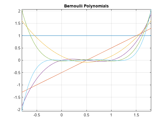
Plot Bernoulli Polynomials
Plot the first six Bernoulli polynomials.
syms x
fplot(bernoulli(0:5, x), [-0.8 1.8])
title('Bernoulli Polynomials')
grid on
Handle Expressions Containing Bernoulli Polynomials
Many functions, such as diff and
expand, handles expressions containing
bernoulli.
Find the first and second derivatives of the Bernoulli polynomial:
syms n x
diff(bernoulli(n,x^2), x)
ans =
2*n*x*bernoulli(n - 1, x^2)
diff(bernoulli(n,x^2), x, x)
ans =
2*n*bernoulli(n - 1, x^2) +...
4*n*x^2*bernoulli(n - 2, x^2)*(n - 1)
Expand these expressions containing the Bernoulli polynomials:
expand(bernoulli(n, x + 3))
ans =
bernoulli(n, x) + (n*(x + 1)^n)/(x + 1) +...
(n*(x + 2)^n)/(x + 2) + (n*x^n)/x
expand(bernoulli(n, 3*x))
ans =
(3^n*bernoulli(n, x))/3 + (3^n*bernoulli(n, x + 1/3))/3 +...
(3^n*bernoulli(n, x + 2/3))/3
Input Arguments
More About
Version History
Introduced in R2014a