Train YOLOX Object Detector Using Synthetic Data
R2026bIn industrial inspection, labeled training data is often scarce due to the rarity of defects and the high cost of expert annotation. This data scarcity makes training accurate deep learning detectors difficult. One solution is to pretrain a detector on synthetic data, and then fine-tune it on the limited real data, thus leveraging the diversity of generated images to teach the detector robust feature representations before adapting it to the real data distribution.
This example shows you how to use synthetic data to improve object detection performance on the BSData pitting defect data set. This example compares these training strategies:
Baseline — Train the detector on only real images.
Synthetic data and real images — Train the detector on synthetic data, then fine-tune it on real images.
By comparing the average precision (AP) between these strategies, you can quantify the benefit of synthetic data augmentation when real annotated data is limited.
Set Up Data Paths
This example uses data prepared using the Generate Synthetic Training Images Using Copy-Paste Augmentation example. Before running this example, run that example to download the BSData data set [1] and generate annotation MAT files. Set the data paths to match the output location from that example.
dataDir = fullfile(tempdir,"BSDataDataset");
sourceImagePath = fullfile(dataDir,"BSData","data");
sourceLabelPath = fullfile(dataDir,"BSData","label");
annotationPath = fullfile(dataDir,"annotations");
Download Pretrained YOLOX Network
By default, this example downloads one version of the YOLOX object detector trained on the real BSData data set, another trained on a synthetic data set, and a third trained on a combination of both. You can use the pretrained networks to run the entire example without waiting for training to complete.
pretrainedDir = fullfile(dataDir,"PretrainedYOLOXDetectorSynthData");
if ~exist(pretrainedDir,"dir")
    unzip("https://ssd.mathworks.com/supportfiles/visualinspection/data/PretrainedYOLOXDetectorSynthData.zip",dataDir);
end
Load Annotated and Unannotated Image Paths
Load the annotation MAT files into the workspace by using the loadImagePaths helper function. Classify images as annotated if they have both a source JPEG and a processed MAT annotation file. Use the remaining images as defect-free backgrounds for synthetic generation.
[annotatedImagePaths,unannotatedImagePaths] = loadImagePaths( ...
    sourceImagePath,sourceLabelPath,annotationPath);
Count the annotated and unannotated source images.
disp("Annotated images: " + numel(annotatedImagePaths))Annotated images: 394
disp("Unannotated (background) images: " + numel(unannotatedImagePaths))Unannotated (background) images: 710
Prepare and Partition Real Data for Training, Validation, and Testing
Split the real annotated data into training, validation, and test sets with a 70/15/15 ratio. Use synthetic data to augment only the training set. The validation and test sets use only real images to provide an unbiased estimate of real-world performance. Set the random number seed to ensure reproducible splits across runs.
rng("default");

numAnnotated = numel(annotatedImagePaths);
numTrain = floor(0.7*numAnnotated);
numVal = floor(0.15*numAnnotated);

shuffledIndices = randperm(numAnnotated);
trainIdx = shuffledIndices(1:numTrain);
valIdx = shuffledIndices(numTrain+1:numTrain+numVal);
testIdx = shuffledIndices(numTrain+numVal+1:end);
For object detection training, you do not need the object masks from the annotations.
returnMasks = false;
Create the training datastore from the real training images.
dsTrainReal = fileDatastore(annotatedImagePaths(trainIdx), ...
    ReadFcn=@(imgPath) readObjectFromMAT(imgPath,annotationPath,returnMasks));
Create the validation datastore.
valDS = fileDatastore(annotatedImagePaths(valIdx), ...
    ReadFcn=@(imgPath) readObjectFromMAT(imgPath,annotationPath,returnMasks));
Create the test datastore.
testDS = fileDatastore(annotatedImagePaths(testIdx), ...
    ReadFcn=@(imgPath) readObjectFromMAT(imgPath,annotationPath,returnMasks));
Display the number of images in each set.
disp("Training set: " + numTrain + " real images")
Training set: 275 real images
disp("Validation set: " + numel(valIdx) + " images")
Validation set: 59 images
disp("Test set: " + numel(testIdx) + " images")
Test set: 60 images
Create Synthetic Training Data Using Copy-Paste Augmentation
Generate 1,000 synthetic training images by inserting defect instances into background images using copy-paste augmentation. Create the object datastore, adding only all of the annotated images, including those in the validation and test sets, to maximize object instance diversity. Use the unannotated images as clean backgrounds onto which you can paste defects. The datastore generates images dynamically during training, so the synthetic data set does not require local storage space.
Include object masks in the defect instance datastore so that copy-paste augmentation can accurately extract defect regions from the source images.
returnObjectMasks = true;

dsObject = fileDatastore(annotatedImagePaths, ...
    ReadFcn=@(imgPath) readObjectFromMAT(imgPath,annotationPath,returnObjectMasks));

dsDestination = imageDatastore(unannotatedImagePaths);

numSyntheticImages = 1000;

dsSynthetic = objectInsertionDatastore(dsDestination,dsObject,numSyntheticImages, ...
    NumObjectsToInsert=[1 3], ...
    ObjectsInSceneMaxOverlap=0.3, ...
    BlendMethod="guidedfilter", ...
    GeometricAugmentation=@() randomAffine2d(Scale=[0.8 1.2], ...
    XReflection=true,YReflection=true,Rotation=[-180 180]), ...
    OutputFormat="ObjectDetection");

disp("Created objectInsertionDatastore with " + numSyntheticImages + " synthetic images")
Created objectInsertionDatastore with 1000 synthetic images
Specify Training Options
Configure the training options for your detector by using the trainingOptions (Deep Learning Toolbox) function to create a TrainingOptionsSGDM object. Use the object across all training experiments to ensure consistent evaluation conditions.
Specify the solver as
"sgdm", creating a stochastic gradient descent with momentum (SGDM) optimizer that enables stable convergence on small data sets.Specify a low initial learning rate with piecewise decay to avoid overshooting when fine-tuning the pretrained weights.
Specify a validation patience of
5to enable early stopping and prevent overfitting, which is especially important when training on small real data sets.Specify the
OutputNetworkname-value argument as"best-validation"to save the checkpoint with the highest validation mAP, rather than the final epoch.Specify the
ObjectiveMetricNamename-value argument as"mAP50", the standard PASCAL VOC evaluation protocol for object detection.
options = trainingOptions("sgdm", ...
    InitialLearnRate=5e-5, ...
    LearnRateSchedule="piecewise", ...
    LearnRateDropFactor=0.98, ...
    LearnRateDropPeriod=1, ...
    MiniBatchSize=32, ...
    MaxEpochs=20, ...
    Shuffle="every-epoch", ...
    VerboseFrequency=1, ...
    ValidationFrequency=25, ...
    ValidationData=valDS, ...
    ValidationPatience=5, ...
    Plots="training-progress", ...
    OutputNetwork="best-validation", ...
    Metrics=mAPObjectDetectionMetric(Name="mAP50"), ...
    L2Regularization=5e-4, ...
    ObjectiveMetricName="mAP50");
Train on Real Images Only
Create a YOLOX object detector by using the yoloxObjectDetector object. Specify the "small-coco" backbone to initialize the network with COCO-pretrained weights for general feature extraction. Then, specify the network input size and class name of the specific defect type, and train the detector on only the real annotated training images by using the trainYOLOXObjectDetector function. This establishes baseline detection accuracy without synthetic data. Set doTraining to true to run the full training process. To instead use the downloaded model pretrained on only the real BSData data set, set doTraining to false.
networkInputSize = [512 512 3];
className = "Pitting";

doTraining = false;
if doTraining
    networkToTrain = yoloxObjectDetector("small-coco",className,InputSize=networkInputSize);
    netReal = trainYOLOXObjectDetector(dsTrainReal,networkToTrain,options);
    modelDateTime = string(datetime("now",Format="yyyy-MM-dd-HH-mm-ss"));
    save(fullfile(dataDir,"trainedYOLOXBSData_" + modelDateTime + ".mat"),"netReal");
else
    pretrained = load(fullfile(dataDir,"trainedYOLOXBSData_Real.mat"));
    netReal = pretrained.net;
end
Evaluate Model
Measure average precision on the test set for the model trained on only real images. Specify a low detection threshold of 0.01 to include all candidate detections in the precision-recall curve, providing an unbiased AP estimate. Use the evaluateObjectDetection function to compute AP at an intersection over union of 0.5, matching the standard PASCAL VOC metric.
reset(testDS)
resultsReal = detect(netReal,testDS,Threshold=0.01);
reset(testDS)
metricsReal = evaluateObjectDetection(resultsReal,testDS,0.5);

disp("=== Evaluation Results: Real Images Only ===")
=== Evaluation Results: Real Images Only ===
summarize(metricsReal)
ans = 1×3 table
    NumObjects    mAPOverlapAvg    mAP0.5
    __________    _____________    ______

        73           0.7603        0.7603
Train Using Synthetic Images and Fine-Tune on Real Images
This two-phase strategy uses synthetic data to learn general defect features and real data to adapt to the actual inspection environment. Phase 1 exposes the network to a large volume of diverse defect appearances and backgrounds, teaching it to recognize pitting defects across various conditions. Phase 2 fine-tunes the detector on the smaller, real data set to close the gap between synthetic and real images.
Phase 1: Train Using Synthetic Images
Train the network on 1,000 synthetic images generated using copy-paste augmentation. The network learns general defect features from the diverse synthetic examples.
if doTraining
    networkToTrain = yoloxObjectDetector("small-coco",className,InputSize=networkInputSize);
    netSynthetic = trainYOLOXObjectDetector(dsSynthetic,networkToTrain,options);
    modelDateTime = string(datetime("now",Format="yyyy-MM-dd-HH-mm-ss"));
    save(fullfile(dataDir,"trainedYOLOXBSData_" + modelDateTime + ".mat"),"netSynthetic");
else
    pretrained = load(fullfile(dataDir,"trainedYOLOXBSData_Synth.mat"));
    netSynthetic = pretrained.net;
end
Phase 2: Fine-Tune Using Real Images
Fine-tune the synthetically pretrained network on real training images. This adapts the learned features to the true data distribution, correcting for subtle differences in texture, lighting, and defect appearance between synthetic and real images.
if doTraining
    netFineTuned = trainYOLOXObjectDetector(dsTrainReal,netSynthetic,options);
    modelDateTime = string(datetime("now",Format="yyyy-MM-dd-HH-mm-ss"));
    save(fullfile(dataDir,"trainedYOLOXBSData_" + modelDateTime + ".mat"),"netFineTuned");
else
    pretrained = load(fullfile(dataDir,"trainedYOLOXBSData_RealSynth.mat"));
    netFineTuned = pretrained.net;
end
Evaluate Model
Measure average precision on the test set for the model trained on synthetic images and fine-tuned on real images. Use the same test set and evaluation protocol as for the baseline, ensuring a direct and fair comparison.
reset(testDS)
resultsFineTuned = detect(netFineTuned,testDS,Threshold=0.01);
reset(testDS)
metricsFineTuned = evaluateObjectDetection(resultsFineTuned,testDS,0.5);

disp("=== Evaluation Results: Synthetic + Fine-tuned ===")
=== Evaluation Results: Synthetic + Fine-tuned ===
summarize(metricsFineTuned)
ans = 1×3 table
    NumObjects    mAPOverlapAvg    mAP0.5
    __________    _____________    _______

        73           0.84602       0.84602
Visualize Detection Results
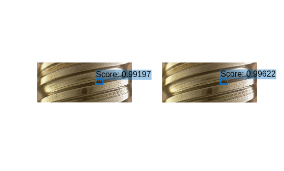
Run inference on a test image using both detectors, and display the results side by side to visually compare detection quality. Specify a detection threshold of 0.3 for visualization to show only confident detections. Compare the two models and observe differences in:
Missed detections, or false negatives
Spurious detections, or false positives
Confidence scores
The synthetic pretrained model typically produces higher-confidence detections with fewer misses than the model trained on only real data.
First, read a test image from the test data set, and run inference using both detectors.
reset(testDS)
testSample = read(testDS);
testImg = testSample{1};
Detect defects in the test image using each model.
[bboxesReal,scoresReal,labelsReal] = detect(netReal,testImg,Threshold=0.3);
[bboxesFT,scoresFT,labelsFT] = detect(netFineTuned,testImg,Threshold=0.3);
Visualize the detection results side by side, overlaying the bounding boxes and confidence scores for each model.
figure
subplot(1,2,1)
title("Real Images Only")
if ~isempty(bboxesReal)
    imshow(testImg)
    showShape("rectangle",bboxesReal, ...
        Label="Score: " + num2str(scoresReal),LabelOpacity=0.4)
else
    imshow(testImg)
end

subplot(1,2,2)
title("Synthetic + Fine-tuned")
if ~isempty(bboxesFT)
    imshow(testImg)
    showShape("rectangle",bboxesFT, ...
        Label="Score: " + num2str(scoresFT),LabelOpacity=0.4)
else
    imshow(testImg)
end
Compare Detection Performance
Compare the average precision scores from both training strategies using the displayAPComparison helper function. The AP improvement quantifies the performance benefit of synthetic pretraining over training on real data alone. Even a modest AP increase translates to fewer missed defects in production inspection.
apReal = metricsReal.ClassMetrics.AP;
apFineTuned = metricsFineTuned.ClassMetrics.AP;

displayAPComparison(apReal,apFineTuned);
=== AP Comparison (IoU = 0.5) ===
Real Images Only:              AP = 0.7603
Synthetic + Fine-tuned:        AP = 0.8460
Improvement:                   AP = +0.0857
Helper Functions
loadImagePaths
Identify annotated and unannotated source images based on the presence of matching MAT annotation files.
function [annotatedImagePaths,unannotatedImagePaths] = loadImagePaths( ...
        sourceImagePath,sourceLabelPath,annotationPath)
labelFiles = dir(fullfile(sourceLabelPath,"*.json"));
imageFiles = dir(fullfile(sourceImagePath,"*.jpg"));
numSourceImages = length(imageFiles);

annotatedImagePaths = {};
for i = 1:numel(labelFiles)
    [~,baseName,~] = fileparts(labelFiles(i).name);
    imgFile = fullfile(sourceImagePath,baseName + ".jpg");
    matFile = fullfile(annotationPath,baseName + ".mat");
    if exist(imgFile,"file") && exist(matFile,"file")
        annotatedImagePaths{end+1} = char(imgFile);
    end
end

annotatedBaseNames = cell(numel(annotatedImagePaths),1);
for i = 1:numel(annotatedImagePaths)
    [~,annotatedBaseNames{i},~] = fileparts(annotatedImagePaths{i});
end

unannotatedImagePaths = {};
for i = 1:numSourceImages
    [~,baseName,~] = fileparts(imageFiles(i).name);
    if ~ismember(baseName,annotatedBaseNames)
        unannotatedImagePaths{end+1} = char(fullfile(sourceImagePath,imageFiles(i).name));
    end
end
end
displayAPComparison
Display a comparison of average precision scores between training strategies.
function displayAPComparison(apReal,apFineTuned)
disp(" ")
disp("=== AP Comparison (IoU = 0.5) ===")
disp("Real Images Only:              AP = " + num2str(apReal{1},"%.4f"))
disp("Synthetic + Fine-tuned:        AP = " + num2str(apFineTuned{1},"%.4f"))
disp("Improvement:                   AP = +" + num2str(apFineTuned{1} - apReal{1},"%.4f"))
end
References
[1] Schlagenhauf, Tobias, and Magnus Landwehr. "Industrial Machine Tool Component Surface Defect Dataset." Data in Brief 39 (December 2021): Article 107643. https://doi.org/10.1016/j.dib.2021.107643.
Copyright 2026 The MathWorks, Inc.

