Contenuto principale

cmorwavf

Complex Morlet wavelet

    Description

    [psi,x] = cmorwavf(lb,ub,n) returns the complex Morlet wavelet psi with time-spread parameter T and center frequency fc both equal to 1. The wavelet is evaluated on an n-point regular grid x for the interval [lb,ub]. The general expression for the complex Morlet wavelet is

    ψ(x)=1Tπexp(2πifcx)exp(x2/ T).

    [psi,x] = cmorwavf(lb,ub,n,T,fc) returns the complex Morlet wavelet with time-spread parameter T and center frequency fc.

    example

    Examples

    collapse all

    Construct a complex-valued Morlet wavelet with a time-spread parameter of 1.5 and a center frequency of 1. Set the effective support to [-6,6] and the number of sample points to 1000.

    N = 1000;
    Lb = -6;
    Ub = 6;
    T = 1.5;
    fc = 1;
    [psi,x] = cmorwavf(Lb,Ub,N,T,fc);

    Plot the real and imaginary parts of the wavelet. Also plot the wavelet magnitude.

    plot(x,real(psi))
    hold on
    plot(x,imag(psi))
    plot(x,abs(psi),LineWidth=2)
    hold off
    grid on
    title("Complex Morlet Wavelet")
    legend("Real","Imaginary","Magnitude")

    Figure contains an axes object. The axes object with title Complex Morlet Wavelet contains 3 objects of type line. These objects represent Real, Imaginary, Magnitude.

    This example shows how the complex Morlet wavelet shape in the frequency domain is affected by the value of the time-spread parameter.

    Create two complex Morlet wavelets in the frequency domain. Both wavelets have a center frequency of 1. Specify a time-spread parameter of 0.5 for one wavelet and a time-spread parameter of 8 for the other wavelet. Plot the wavelets in the frequency domain.

    f = -4:.01:4;  
    Fc = 1;      % center frequency
    T1 = 0.5;   % time-spread parameter
    T2 = 8;     % time-spread parameter
    psihat1 = exp(-pi^2*T1*(f-Fc).^2);  
    psihat2 = exp(-pi^2*T2*(f-Fc).^2);  
    plot(f,psihat1)  
    hold on
    plot(f,psihat2)
    hold off
    title("Complex Morlet Wavelets in Frequency Domain")
    legend("Time-spread = 0.5","Time-spread = 8",Location="northwest")

    Figure contains an axes object. The axes object with title Complex Morlet Wavelets in Frequency Domain contains 2 objects of type line. These objects represent Time-spread = 0.5, Time-spread = 8.

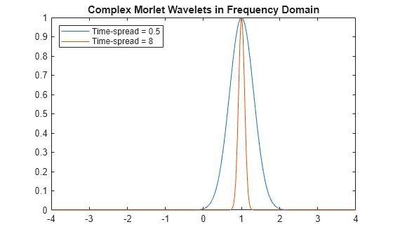
    The time-spread parameter for the complex Morlet wavelet is proportional to the inverse of the variance in frequency. Therefore, increasing the time-spread parameter increases the concentration of energy around the center frequency.

    Input Arguments

    collapse all

    Left endpoint of the closed interval, specified as a scalar. lb is strictly less than ub.

    Right endpoint of the closed interval, specified as a scalar. ub is strictly greater than ub.

    Number of regularly spaced points in the interval [lb,ub], specified as a positive integer.

    Time-spread parameter, specified as a positive scalar. The time-spread parameter controls the spread in the time domain and the corresponding energy spread (bandwidth) in the frequency domain. The time-spread parameter is proportional to the inverse of the variance in the frequency domain. It is two times the time variance of the wavelet.

    • Increasing the time-spread parameter concentrates the wavelet energy around the center frequency and increases the spread of the wavelet in time.

    • Decreasing the time-spread parameter reduces its spread in time and thereby increases the spread in frequency.

    The time-spread parameter does not affect the center frequency. When converting from scale to frequency, only the center frequency affects the frequency values. The energy spread or time-spread parameter affects how localized the wavelet is in the frequency domain.

    Center frequency, specified as a positive scalar.

    Output Arguments

    collapse all

    Complex Morlet wavelet, returned as a complex-valued 1-by-n vector.

    Sample points where the complex Morlet wavelet is evaluated, returned as a 1-by-n vector. The sample points are evenly distributed between lb and ub.

    References

    [1] Teolis, Anthony. Computational Signal Processing with Wavelets. Boston, MA: Birkhäuser Boston, 1998. https://doi.org/10.1007/978-1-4612-4142-3.

    Version History

    Introduced before R2006a

    See Also